Object Detection and Classification using R-CNNs

In this post, I’ll describe in detail how R-CNN (Regions with CNN features), a recently introduced deep learning based object detection and classification method works. R-CNN’s have proved highly effective in detecting and classifying objects in natural images, achieving mAP scores far higher than previous techniques. The R-CNN method is described in the following series of papers by Ross Girshick et al.

1. R-CNN (https://arxiv.org/abs/1311.2524)
2. Fast R-CNN (https://arxiv.org/abs/1504.08083)
3. Faster R-CNN (https://arxiv.org/abs/1506.01497)

This post describes the final version of the R-CNN method described in the last paper. I considered at first to describe the evolution of the method from its first introduction to the final version, however that turned out to be a very ambitious undertaking. I settled on describing the final version in detail.

Fortunately, there are many implementations of the R-CNN algorithm available on the web in TensorFlow, PyTorch and other machine learning libraries. I used the following implementation:

https://github.com/ruotianluo/pytorch-faster-rcnn

Much of the terminology used in this post (for example the names of different layers) follows the terminology used in the code. Understanding the information presented in this post should make it much easier to follow the PyTorch implementation and make your own modifications.

Post Organization

• Section 1 – Image Pre-Processing: In this section, we’ll describe the pre-processing steps that are applied to an input image. These steps include subtracting a mean pixel value and scaling the image. The pre-processing steps must be identical between training and inference
• Section 2 – Network Organization: In this section, we’ll describe the three main components of the network – the “head” network, the region proposal network (RPN) and the classification network.
• Section 3 – Implementation Details (Training): This is the longest section of the post and describes in detail the steps involved in training a R-CNN network 
• Section 4 – Implementation Details (Inference): In this section, we’ll describe the steps involved during inference – i.e., using the trained R-CNN network to identify promising regions and classify the objects in those regions.
• Appendix: Here we’ll cover the details of some of the frequently used algorithms during the operation of a R-CNN such as non-maximum suppression and the details of the Resnet 50 architecture.

Image Pre-Processing

The following pre-processing steps are applied to an image before it is sent through the network. These steps must be identical for both training and inference. The mean vector (, one number corresponding to each color channel) is not the mean of the pixel values in the current image but a configuration value that is identical across all training and test images.

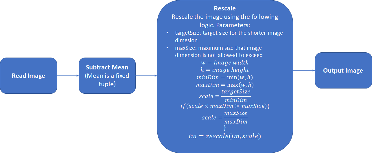
The default values for and parameters are 600 and 1000 respectively.

Network Organization

A R-CNN uses neural networks to solve two main problems:

• Identify promising regions (Region of Interest – ROI) in an input image that are likely to contain foreground objects
• Compute the object class probability distribution of each ROI – i.e., compute the probability that the ROI contains an object of a certain class. The user can then select the object class with the highest probability as the classification result.

R-CNNs consist of three main types of networks:

1. Head
2. Region Proposal Network (RPN)
3. Classification Network

R-CNNs use the first few layers of a pre-trained network such as ResNet 50 to identify promising features from an input image. Using a network trained on one dataset on a different problem is possible because neural networks exhibit “transfer learning” (https://arxiv.org/abs/1411.1792). The first few layers of the network learn to detect general features such as edges and color blobs that are good discriminating features across many different problems. The features learnt by the later layers are higher level, more problem specific features. These layers can either be removed or the weights for these layers can be fine-tuned during back-propagation. The first few layers that are initialized from a pre-trained network constitute the “head” network. The convolutional feature maps produced by the head network are then passed through the Region Proposal Network (RPN) which uses a series of convolutional and fully connected layers to produce promising ROIs that are likely to contain a foreground object (problem 1 mentioned above). These promising ROIs are then used to crop out corresponding regions from the feature maps produced by the head network. This is called “Crop Pooling”. The regions produced by crop pooling are then passed through a classification network which learns to classify the object contained in each ROI.

As an aside, you may notice that weights for a ResNet are initialized in a curious way:

If you are interested in learning more about why this method works, read my post about initializing weights for convolutional and fully connected layers.

Network Architecture

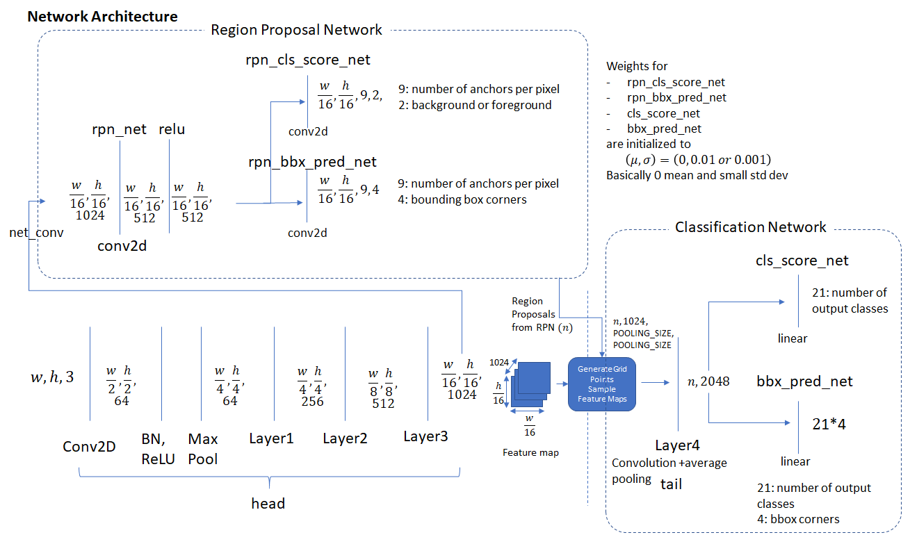
The diagram below shows the individual components of the three network types described above. We show the dimensions of the input and output of each network layer which assists in understanding how data is transformed by each layer of the network. and represent the width and height of the input image (after pre-processing).

 

Implementation Details: Training

In this section, we’ll describe in detail the steps involved in training a R-CNN. Once you understand how training works, understanding inference is a lot easier as it simply uses a subset of the steps involved in training. The goal of training is to adjust the weights in the RPN and Classification network and fine-tune the weights of the head network (these weights are initialized from a pre-trained network such as ResNet). Recall that the job of the RPN network is to produce promising ROIs and the job of the classification network to assign object class scores to each ROI. Therefore, to train these networks, we need the corresponding ground truth i.e., the coordinates of the bounding boxes around the objects present in an image and the class of those objects. This ground truth comes from free to use image databases that come with an annotation file for each image. This annotation file contains the coordinates of the bounding box and the object class label for each object present in the image (the object classes are from a list of pre-defined object classes). These image databases have been used to support a variety of object classification and detection challenges. Two commonly used databases are:

• PASCAL VOC: The VOC 2007 database contains 9963 training/validation/test images with 24,640 annotations for 20 object classes.
  • Person: person
  • Animal: bird, cat, cow, dog, horse, sheep
  • Vehicle: aeroplane, bicycle, boat, bus, car, motorbike, train
  • Indoor: bottle, chair, dining table, potted plant, sofa, tv/monitor

• COCO (Common Objects in Context): The COCO dataset is much larger. It contains > 200K labelled images with 90 object categories.

I used the smaller PASCAL VOC 2007 dataset for my training. R-CNN is able to train both the region proposal network and the classification network in the same step.

Let’s take a moment to go over the concepts of “bounding box regression coefficients” and “bounding box overlap” that are used extensively in the remainder of this post.

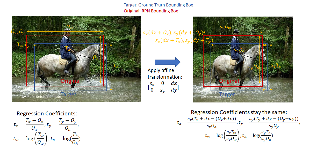
• Bounding Box Regression Coefficients (also referred to as “regression coefficients” and “regression targets”): One of the goals of R-CNN is to produce good bounding boxes that closely fit object boundaries. R-CNN produces these bounding boxes by taking a given bounding box (defined by the coordinates of the top left corner, width and height) and tweaking its top left corner, width and height by applying a set of “regression coefficients”. These coefficients are computed as follows (Appendix C of (https://arxiv.org/pdf/1311.2524.pdf). Let the x, y coordinates of the top left corner of the target and original bounding box be denoted by respectively and the width/height of the target and original bounding box by respectively. Then, the regression targets (coefficients of the function that transform the original bounding box to the target box) are given as:
  • . This function is readily invertible, i.e., given the regression coefficients and coordinates of the top left corner and the width and height of the original bounding box, the top left corner and width and height of the target box can be easily calculated. Note the regression coefficients are invariant to an affine transformation with no shear. This is an important point as while calculating the classification loss, the target regression coefficients are calculated in the original aspect ratio while the classification network output regression coefficients are calculated after the ROI pooling step on square feature maps (1:1 aspect ratio). This will become clearer when we discuss classification loss below.

    

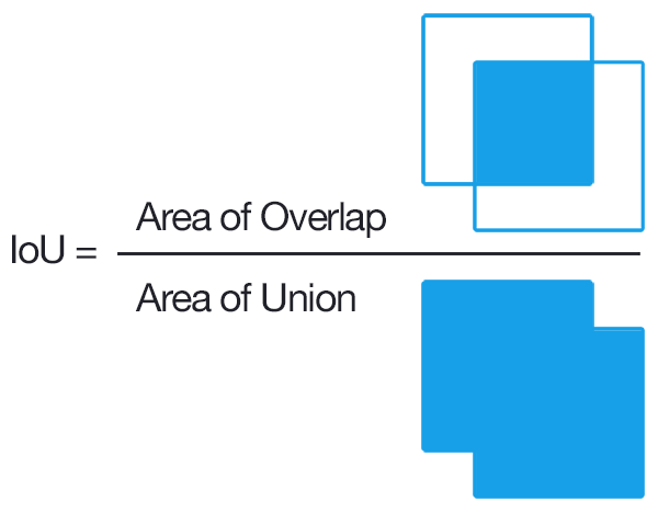
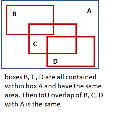
• Intersection over Union (IoU) Overlap: We need some measure of how close a given bounding box is to another bounding box that is independent of the units used (pixels etc) to measure the dimensions of a bounding box. This measure should be intuitive (two coincident bounding boxes should have an overlap of 1 and two non-overlapping boxes should have an overlap of 0) and fast and easy to calculate. A commonly used overlap measure is the “Intersection over Union (IoU) overlap, calculated as shown below.
  

  

 

With these preliminaries out of the way, lets now dive into the implementation details for training a R-CNN. In the software implementation, R-CNN execution is broken down into several layers, as shown below. A layer encapsulates a sequence of logical steps that can involve running data through one of the neural networks and other steps such as comparing overlap between bounding boxes, performing non-maxima suppression etc.

 

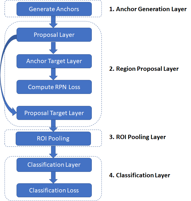
• Anchor Generation Layer: This layer generates a fixed number of “anchors” (bounding boxes) by first generating 9 anchors of different scales and aspect ratios and then replicating these anchors by translating them across uniformly spaced grid points spanning the input image.
• Proposal Layer: Transform the anchors according to the bounding box regression coefficients to generate transformed anchors. Then prune the number of anchors by applying non-maximum suppression (see Appendix) using the probability of an anchor being a foreground region
• Anchor Target Layer: The goal of the anchor target layer is to produce a set of “good” anchors and the corresponding foreground/background labels and target regression coefficients to train the Region Proposal Network. The output of this layer is only used to train the RPN network and is not used by the classification layer. Given a set of anchors (produced by the anchor generation layer, the anchor target layer identifies promising foreground and background anchors. Promising foreground anchors are those whose overlap with some ground truth box is higher than a threshold. Background boxes are those whose overlap with any ground truth box is lower than a threshold. The anchor target layer also outputs a set of bounding box regressors i.e., a measure of how far each anchor target is from the closest bounding box. These regressors only make sense for the foreground boxes as there is no notion of “closest bounding box” for a background box.
• RPN Loss: The RPN loss function is the metric that is minimized during optimization to train the RPN network. The loss function is a combination of:
  • The proportion of bounding boxes produced by RPN that are correctly classified as foreground/background
  • Some distance measure between the predicted and target regression coefficients.
• Proposal Target Layer: The goal of the proposal target layer is to prune the list of anchors produced by the proposal layer and produce class specific bounding box regression targets that can be used to train the classification layer to produce good class labels and regression targets
• ROI Pooling Layer: Implements a spatial transformation network that samples the input feature map given the bounding box coordinates of the region proposals produced by the proposal target layer. These coordinates will generally not lie on integer boundaries, thus interpolation based sampling is required.
• Classification Layer: The classification layer takes the output feature maps produced by the ROI Pooling Layer and passes them through a series of convolutional layers. The output is fed through two fully connected layers. The first layer produces the class probability distribution for each region proposal and the second layer produces a set of class specific bounding box regressors.
• Classification Loss: Similar to RPN loss, classification loss is the metric that is minimized during optimization to train the classification network. During back propagation, the error gradients flow to the RPN network as well, so training the classification layer modifies the weights of the RPN network as well. We’ll have more to say about this point later. The classification loss is a combination of:
  • The proportion of bounding boxes produced by RPN that are correctly classified (as the correct object class)
  • Some distance measure between the predicted and target regression coefficients.

We’ll now go through each of these layers in detail.

Anchor Generation Layer

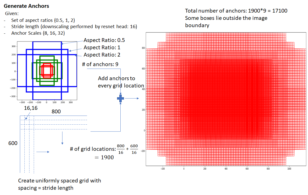
The anchor generation layer produces a set of bounding boxes (called “anchor boxes”) of varying sizes and aspect ratios spread all over the input image. These bounding boxes are the same for all images i.e., they are agnostic of the content of an image. Some of these bounding boxes will enclose foreground objects while most won’t. The goal of the RPN network is to learn to identify which of these boxes are good boxes – i.e., likely to contain a foreground object and to produce target regression coefficients, which when applied to an anchor box turns the anchor box into a better bounding box (fits the enclosed foreground object more closely).

The diagram below demonstrates how these anchor boxes are generated.

Region Proposal Layer

Object detection methods need as input a “region proposal system” that produces a set of sparse (for example selective search (http://link.springer.com/article/10.1007/s11263-013-0620-5")) or a dense (for example features used in deformable part models (https://doi.org/10.1109/TPAMI.2009.167")) set of features. The first version of the R-CNN system used the selective search method for generating region proposal. In the current version (known as “Faster R-CNN”), a “sliding window” based technique (described in the previous section) is used to generate a set of dense candidate regions and then a neural network driven region proposal network is used to rank region proposals according to the probability of a region containing a foreground object. The region proposal layer has two goals:

• From a list of anchors, identify background and foreground anchors
• Modify the position, width and height of the anchors by applying a set of “regression coefficients” to improve the quality of the anchors (for example, make them fit the boundaries of objects better)

The region proposal layer consists of a Region Proposal Network and three layers – Proposal Layer, Anchor Target Layer and Proposal Target Layer. These three layers are described in detail in the following sections.

Region Proposal Network

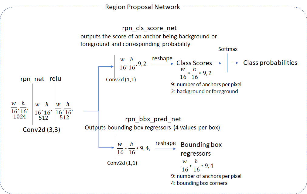
The region proposal layer runs feature maps produced by the head network through a convolutional layer (called rpn_net in code) followed by RELU. The output of rpn_net is run through two (1,1) kernel convolutional layers to produce background/foreground class scores and probabilities and corresponding bounding box regression coefficients. The stride length of the head network matches the stride used while generating the anchors, so the number of anchor boxes are in 1-1 correspondence with the information produced by the region proposal network (number of anchor boxes = number of class scores = number of bounding box regression coefficients = )

Proposal Layer

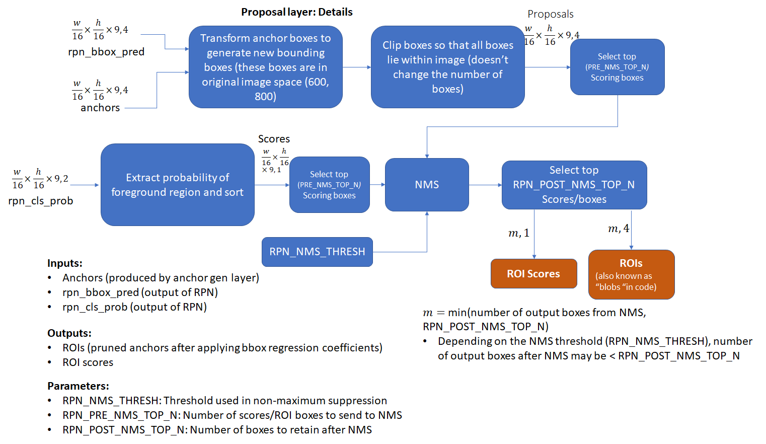
The proposal layer takes the anchor boxes produced by the anchor generation layer and prunes the number of boxes by applying non-maximum suppression based on the foreground scores (see appendix for details). It also generates transformed bounding boxes by applying the regression coefficients generated by the RPN to the corresponding anchor boxes.

 Anchor Target Layer

The goal of the anchor target layer is to select promising anchors that can be used to train the RPN network to:

1. distinguish between foreground and background regions and
2. generate good bounding box regression coefficients for the foreground boxes.

It is useful to first look at how the RPN Loss is calculated. This will reveal the information needed to calculate the RPN loss which makes it easy to follow the operation of the Anchor Target Layer.

Calculating RPN Loss

Remember the goal of the RPN layer is to generate good bounding boxes. To do so from a set of anchor boxes, the RPN layer must learn to classify an anchor box as background or foreground and calculate the regression coefficients to modify the position, width and height of a foreground anchor box to make it a “better” foreground box (fit a foreground object more closely). RPN Loss is formulated in such a way to encourage the network to learn this behaviour.

RPN loss is a sum of the classification loss and bounding box regression loss. The classification loss uses cross entropy loss to penalize incorrectly classified boxes and the regression loss uses a function of the distance between the true regression coefficients (calculated using the closest matching ground truth box for a foreground anchor box) and the regression coefficients predicted by the network (see rpn_bbx_pred_net in the RPN network architecture diagram).

Classification Loss:

cross_entropy(predicted _class, actual_class)

Bounding Box Regression Loss:

Sum over the regression losses for all foreground anchors. Doing this for background anchors doesn’t make sense as there is no associated ground truth box for a background anchor

This shows how the regression loss for a given foreground anchor is calculated. We take the difference between the predicted (by the RPN) and target (calculated using the closest ground truth box to the anchor box) regression coefficients. There are four components – corresponding to the coordinates of the top left corner and the width/height of the bounding box. The smooth L1 function is defined as follows:

Here is chosen arbitrarily (set to 3 in my code). Note that in the python implementation, a mask array for the foreground anchors (called “bbox_inside_weights”) is used to calculate the loss as a vector operation and avoid for-if loops.

Thus, to calculate the loss we need to calculate the following quantities:

1. Class labels (background or foreground) and scores for the anchor boxes
2. Target regression coefficients for the foreground anchor boxes

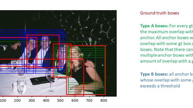
We’ll now follow the implementation of the anchor target layer to see how these quantities are calculated. We first select the anchor boxes that lie within the image extent. Then, good foreground boxes are selected by first computing the IoU (Intersection over Union) overlap of all anchor boxes (within the image) with all ground truth boxes. Using this overlap information, two types of boxes are marked as foreground:

1. type A: For each ground truth box, all foreground boxes that have the max IoU overlap with the ground truth box
2. type B: Anchor boxes whose maximum overlap with some ground truth box exceeds a threshold

these boxes are shown in the image below:

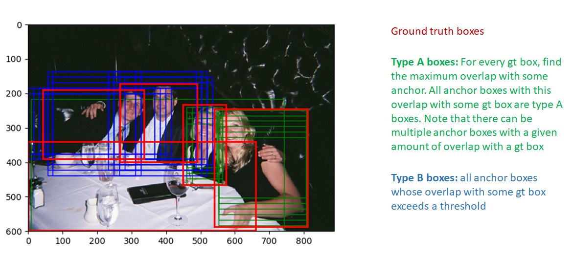
Note that only anchor boxes whose overlap with some ground truth box exceeds a threshold are selected as foreground boxes. This is done to avoid presenting the RPN with the “hopeless learning task” of learning the regression coefficients of boxes that are too far from the best match ground truth box. Similarly, boxes whose overlap are less than a negative threshold are labeled background boxes. Not all boxes that are not foreground boxes are labeled background. Boxes that are neither foreground or background are labeled “don’t care”. These boxes are not included in the calculation of RPN loss.

There are two additional thresholds related to the total number of background and foreground boxes we want to achieve and the fraction of this number that should be foreground. If the number of foreground boxes that pass the test exceeds the threshold, we randomly mark the  excess foreground boxes to “don’t care”. Similar logic is applied to the background boxes.

Next, we compute bounding box regression coefficients between the foreground boxes and the corresponding ground truth box with maximum overlap. This is easy and one just needs to follow the formula to calculate the regression coefficients.

This concludes our discussion of the anchor target layer. To recap, let’s list the parameters and input/output for this layer:

Parameters:

• TRAIN.RPN_POSITIVE_OVERLAP: Threshold used to select if an anchor box is a good foreground box (Default: 0.7)
• TRAIN.RPN_NEGATIVE_OVERLAP: If the max overlap of a anchor from a ground truth box is lower than this thershold, it is marked as background. Boxes whose overlap is > than RPN_NEGATIVE_OVERLAP but < RPN_POSITIVE_OVERLAP are marked “don’t care”.(Default: 0.3)
• TRAIN.RPN_BATCHSIZE: Total number of background and foreground anchors (default: 256)
• TRAIN.RPN_FG_FRACTION: fraction of the batch size that is foreground anchors (default: 0.5). If the number of foreground anchors found is larger than TRAIN.RPN_BATCHSIZE TRAIN.RPN_FG_FRACTION, the excess (indices are selected randomly) is marked “don’t care”.

Input:

• RPN Network Outputs (predicted foreground/background class labels, regression coefficients)
• Anchor boxes (generated by the anchor generation layer)
• Ground truth boxes

Output

• Good foreground/background boxes and associated class labels
• Target regression coefficients

The other layers, proposal target layer, ROI Pooling layer and classification layer are meant to generate the information needed to calculate classification loss. Just as we did for the anchor target layer, let’s first look at how classification loss is calculated and what information is needed to calculate it

Calculating Classification Layer Loss

Similar to the RPN Loss, classification layer loss has two components – classification loss and bounding box regression loss

The key difference between the RPN layer and the classification layer is that while the RPN layer dealt with just two classes – foreground and background, the classification layer deals with all the object classes (plus background) that our network is being trained to classify.

The classification loss is the cross entropy loss with the true object class and predicted class score as the parameters. It is calculated as shown below.

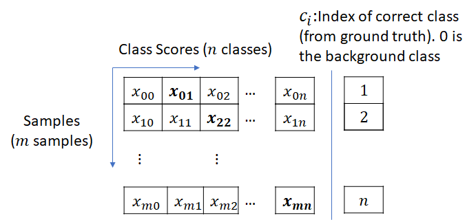
The bounding box regression loss is also calculated similar to the RPN except now the regression coefficients are class specific. The network calculates regression coefficients for each object class. The target regression coefficients are obviously only available for the correct class which is the object class of the ground truth bounding box that has the maximum overlap with a given anchor box. While calculating the loss, a mask array which marks the correct object class for each anchor box is used. The regression coefficients for the incorrect object classes are ignored. This mask array allows the computation of loss to be a matrix multiplication as opposed to requiring a for-each loop.

Thus the following quantities are needed to calculate classification layer loss:

1. Predicted class labels and bounding box regression coefficients (these are outputs of the classification network)
2. class labels for each anchor box
3. Target bounding box regression coefficients

Let’s now look at how these quantities are calculated in the proposal target and classification layers.

Proposal Target Layer

The goal of the proposal target layer is to select promising ROIs from the list of ROIs output by the proposal layer. These promising ROIs will be used to perform crop pooling from the feature maps produced by the head layer and passed to the rest of the network (head_to_tail) that calculates predicted class scores and box regression coefficients.

Similar to the anchor target layer, it is important to select good proposals (those that have significant overlap with gt boxes) to pass on to the classification layer. Otherwise, we’ll be asking the classification layer to learn a “hopeless learning task”.

The proposal target layer starts with the ROIs computed by the proposal layer. Using the max overlap of each ROI with all ground truth boxes, it categorizes the ROIs into background and foreground ROIs. Foreground ROIs are those for which max overlap exceeds a threshold (TRAIN.FG_THRESH, default: 0.5). Background ROIs are those whose max overlap falls between TRAIN.BG_THRESH_LO and TRAIN.BG_THRESH_HI (default 0.1, 0.5 respectively). This is an example of “hard negative mining” used to present difficult background examples to the classifier.

There is some additional logic that tries to make sure that the total number of foreground and background region is constant. In case too few background regions are found, it tries to fill in the batch by randomly repeating some background indices to make up for the shortfall.

Next, bounding box target regression targets are computed between each ROI and the closest matching ground truth box (this includes the background ROIs also, as an overlapping ground truth box exists for these ROIs also). These regression targets are expanded for all classes as shown in the figure below.

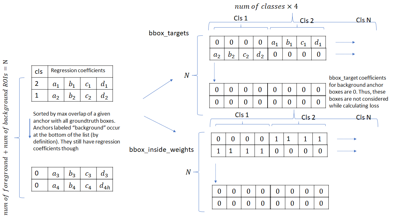
the bbox_inside_weights array acts as a mask. It is 1 only for the correct class for each foreground ROI. It is zero for the background ROIs as well. Thus, while computing the bounding box regression component of the classification layer loss, only the regression coefficients for the foreground regions are taken into account. This is not the case for the classification loss – the background ROIs are included as well as they belong to the “background” class.

Input:

• ROIs produced by the proposal layer
• ground truth information

Output:

• Selected foreground and background ROIs that meet overlap criteria.
• Class specific target regression coefficients for the ROIs

Parameters:

• TRAIN.FG_THRESH: (default: 0.5) Used to select foreground ROIs. ROIs whose max overlap with a ground truth box exceeds FG_THRESH are marked foreground
• TRAIN.BG_THRESH_HI: (default 0.5)
• TRAIN.BG_THRESH_LO: (default 0.1) These two thresholds are used to select background ROIs. ROIs whose max overlap falls between BG_THRESH_HI and BG_THRESH_LO are marked background
• TRAIN.BATCH_SIZE: (default 128) Maximum number of foreground and background boxes selected.
• TRAIN.FG_FRACTION: (default 0.25). Number of foreground boxes can’t exceed BATCH_SIZE*FG_FRACTION

Crop Pooling

Proposal target layer produces promising ROIs for us to classify along with the associated class labels and regression coefficients that are used during training. The next step is to extract the regions corresponding to these ROIs from the convolutional feature maps produced by the head network. The extracted feature maps are then run through the rest of the network (“tail” in the network diagram shown above) to produce object class probability distribution and regression coefficients for each ROI. The job of the Crop Pooling layer is to perform region extraction from the convolutional feature maps.

The key ideas behind crop pooling are described in the paper on “Spatial Transformation Networks” (https://arxiv.org/pdf/1506.02025.pdf). The goal is to apply a warping function (described by a affine transformation matrix) to an input feature map to output a warped feature map. This is shown in the figure below

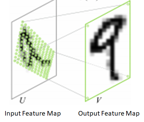
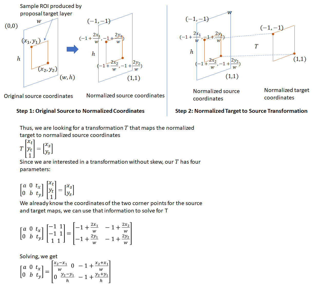
There are two steps involved in crop pooling:

1. For a set of target coordinates, apply the given affine transformation to produce a grid of source coordinates.
   . Here are height/width normalized coordinates (similar to the texture coordinates used in graphics), so .
2. In the second step, the input (source) map is sampled at the source coordinates to produce the output (destination) map. In this step, each coordinate defines the spatial location in the input where a sampling kernel (for example bi-linear sampling kernel) is applied to get the value at a particular pixel in the output feature map.

The sampling methodology described in the spatial transformation gives a differentiable sampling mechanism allowing for loss gradients to flow back to the input feature map and the sampling grid coordinates.

Fortunately, crop pooling is implementated in PyTorch and the API consists of two functions that mirror these two steps. torch.nn.functional.affine_grid takes an affine transformation matrix and produces a set of sampling coordinates and torch.nn.functional.grid_sample samples the grid at those coordinates. Back-propagating gradients during the backward step is handled automatically by pyTorch.

To use crop pooling, we need to do the following:

1. Divide the ROI coordinates by the stride length of the “head” network. The coordinates of the ROIs produced by the proposal target layer are in the original image space (! 800 600). To bring these coordinates into the space of the output feature maps produced by “head”, we must divide them by the stride length (16 in the current implementation).
2. To use the API shown above, we need the affine transformation matrix. This affine transformation matrix is computed as shown below
3. We also need the number of points in the and dimensions on the target feature map. This is provided by the configuration parameter cfg.POOLING_SIZE (default 7). Thus, during crop pooling, non-square ROIs are used to crop out regions from the convolution feature map which are warped to square windows of constant size. This warping must be done as the output of crop pooling is passed to further convolutional and fully connected layers which need input of a fixed dimension.

   

Classification Layer

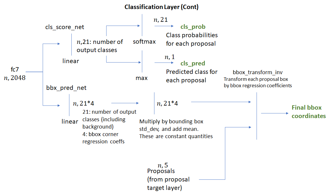
The crop pooling layer takes the ROI boxes output by the proposal target layer and the convolutional feature maps output by the “head” network and outputs square feature maps. The feature maps are then passed through layer 4 of ResNet following by average pooling along the spatial dimensions. The result (called “fc7” in code) is a one-dimensional feature vector for each ROI. This process is shown below.

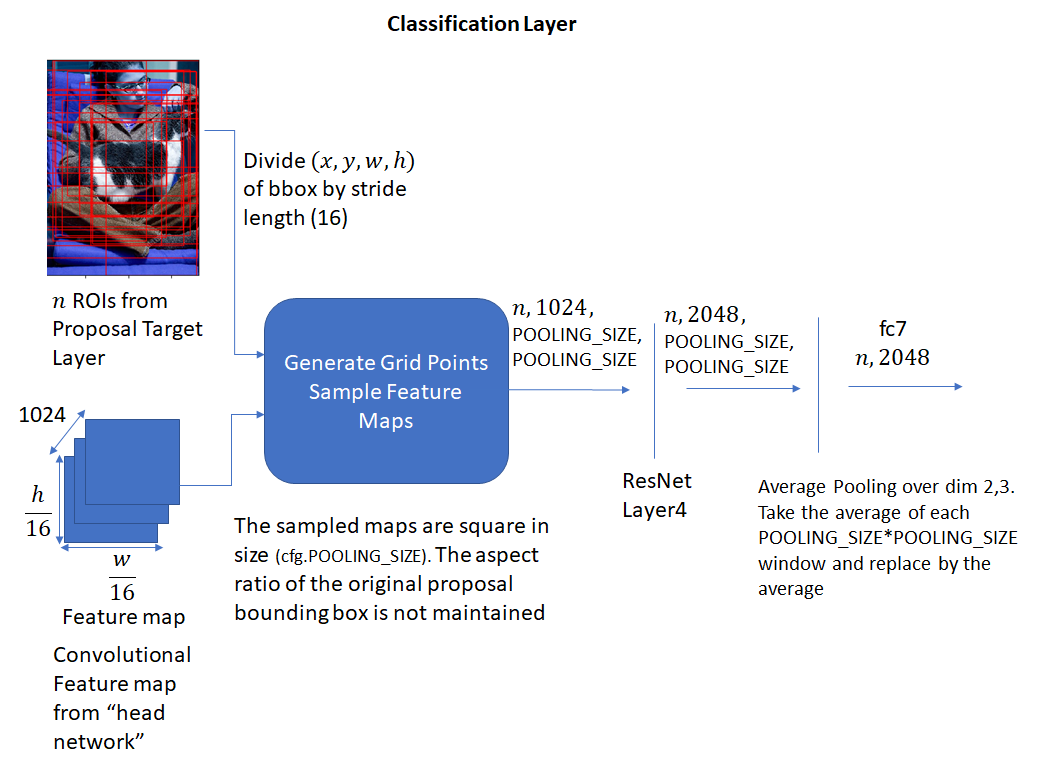
The feature vector is then passed through two fully connected layers – bbox_pred_net and cls_score_net. The cls_score_net layer produces the class scores for each bounding box (which can be converted into probabilities by applying softmax). The bbox_pred_net layer produces the class specific bounding box regression coefficients which are combined with the original bounding box coordinates produced by the proposal target layer to produce the final bounding boxes. These steps are shown below.

It’s good to recall the difference between the two sets of bounding box regression coefficients – one set produced by the RPN network and the second set produced by the classification network. The first set is used to train the RPN layer to produce good foreground bounding boxes (that fit more tightly around object boundaries). The target regression coefficients i.e., the coefficients needed to align a ROI box with its closest matching ground truth bounding box are generated by the anchor target layer. It is difficult to identify precisely how this learning takes place, but I’d imagine the RPN convolutional and fully connected layers learn how to interpret the various image features generated by the neural network into deciphering good object bounding boxes. When we consider Inference in the next section, we’ll see how these regression coefficients are used.

The second set of bounding box coefficients is generated by the classification layer. These coefficients are class specific, i.e., one set of coefficients are generated per object class for each ROI box. The target regression coefficients for these are generated by the proposal target layer. Note that the classification network operates on square feature maps that are a result of the affine transformation (described above) applied to the head network output. However since the regression coefficients are invariant to an affine transformation with no shear, the target regression coefficients computed by the proposal target layer can be compared with those produced by the classification network and act as a valid learning signal. This point seems obvious in hindsight, but took me some time to understand.

It is interesting to note that while training the classification layer, the error gradients propagate to the RPN network as well. This is because the ROI box coordinates used during crop pooling are themselves network outputs as they are a result of applying the regression coefficients generated by the RPN network to the anchor boxes. During back-propagation, the error gradients will propagate back through the crop-pooling layer to the RPN layer. Calculating and applying these gradients would be quite tricky to implement, however thankfully the crop pooling API is provided by PyTorch as a built-in module and the details of calculating and applying the gradients are handled internally. This point is discussed in Section 3.2 (iii) of the Faster RCNN paper  (https://arxiv.org/abs/1506.01497).

Implementation Details: Inference

The steps carried out during inference are shown below

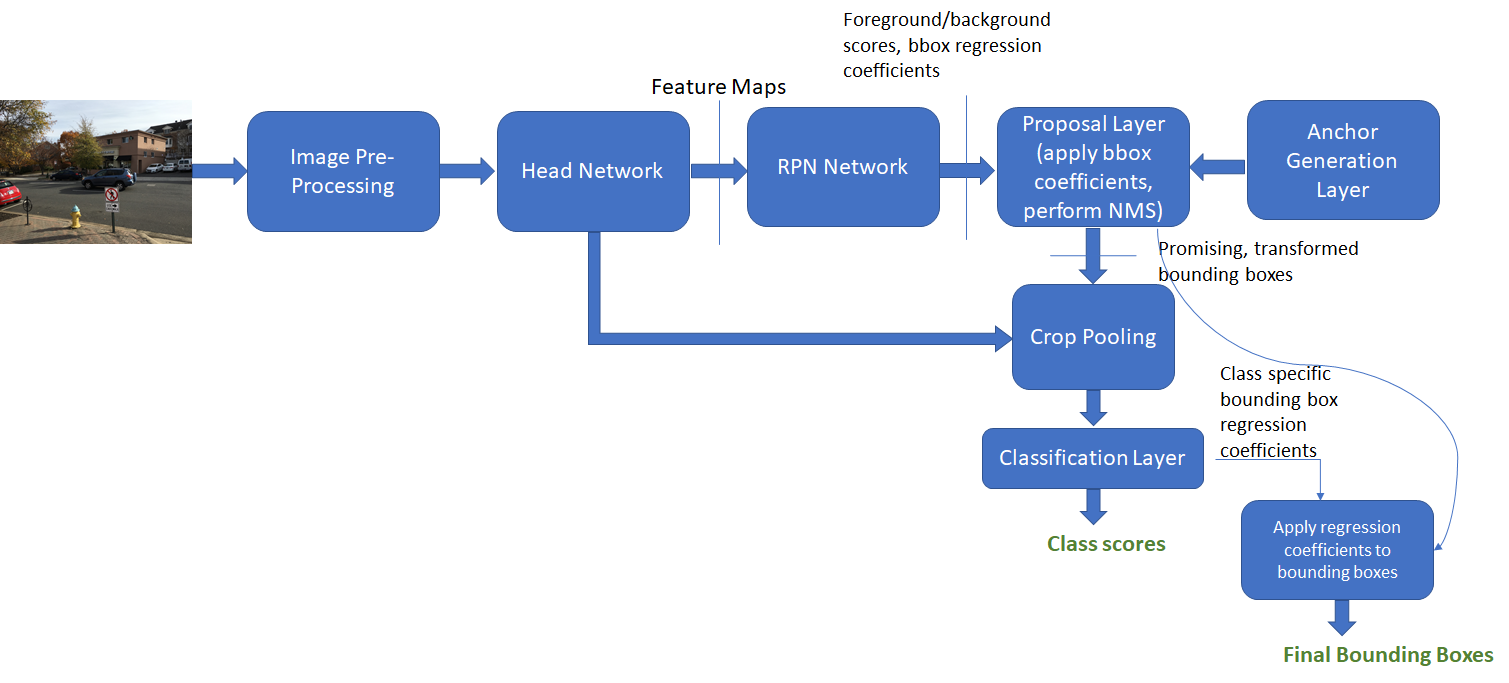
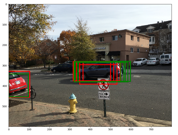
Anchor target and proposal target layers are not used. The RPN network is supposed to have learnt how to classify the anchor boxes into background and foreground boxes and generate good bounding box coefficients. The proposal layer simply applies the bounding box coefficients to the top ranking anchor boxes and performs NMS to eliminate boxes with a large amount of overlap. The output of these steps are shown below for additional clarity. The resulting boxes are sent to the classification layer where class scores and class specific bounding box regression coefficients are generated.

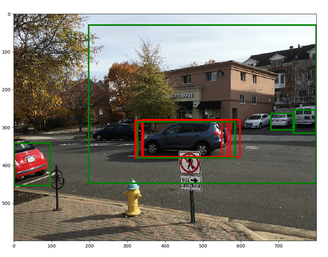
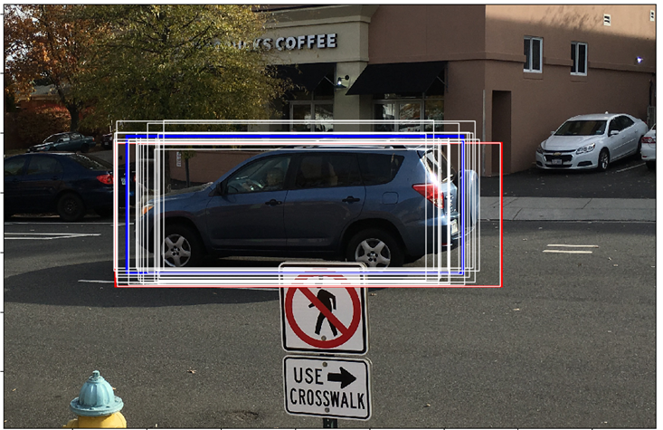
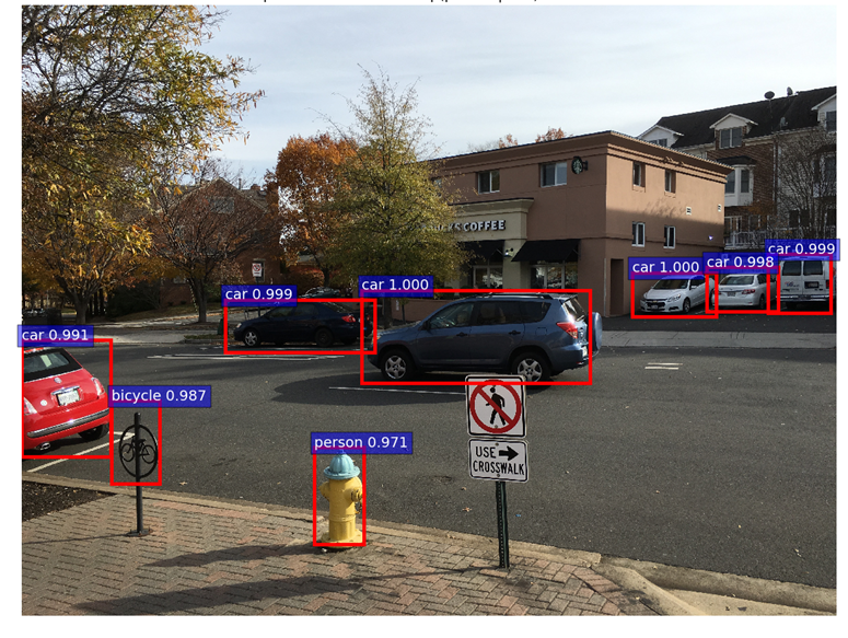
For showing the final classification results, we apply another round of NMS and apply an object detection threshold to the class scores. We then draw all transformed bounding boxes corresponding to the ROIs that meet the detection threshold. The result is shown below.

Appendix

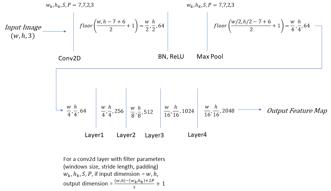
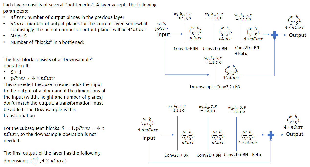
ResNet 50 Network Architecture

Non-Maximum Suppression (NMS)

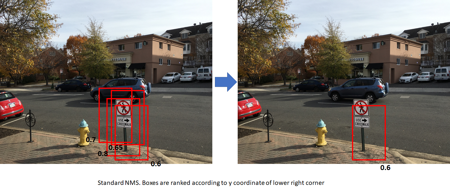
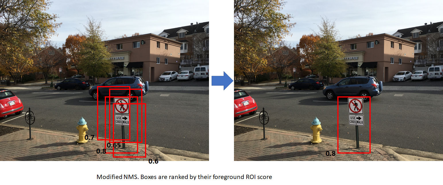
Non-maximum suppression is a technique used to reduce the number of candidate boxes by eliminating boxes that overlap by an amount larger than a threhold. The boxes are first sorted by some criteria (usually the y coordinate of the bottom right corner). We then go through the list of boxes and suppress those boxes whose IoU overlap with the box under consideration exceeds a threshold. Sorting the boxes by the y coordinate results in the lowest box among a set of overlapping boxes being retained. This may not always be the desired outcome. NMS used in R-CNN sorts the boxes by the foreground score. This results in the box with the highest score among a set of overlapping boxes being retained. The figures below show the difference between the two approaches. The numbers in black are the foreground scores for each box. The image on the right shows the result of applying NMS to the image on left. The first figure uses standard NMS (boxes are ranked by y coordinate of bottom right corner). This results in the box with a lower score being retained. The second figure uses modified NMS (boxes are ranked by foreground scores). This results in the box with the highest foreground score being retained, which is more desirable. In both cases, the overlap between the boxes is assumed to be higher than the NMS overlap threhold.

 

 

Bibliography