Kernel SHAP

In this post, I will provide the math for eliminating the constraint on the sum of Shap (SHapley Additive exPlanations) values in the KernelSHAP algorithm as mentioned in this paper, along with the Python implementation. Although KernelSHAP implementation is already available in the Python Shap package, my implementation is much simpler and easier to understand and provides a distributed implementation for computing Shap values for multiple data instances. The code is available here.

If you have no idea what I just said, I recommend reading the excellent intuitive explanation of Shapley values in this book. Here, I will outline two points that can be easy to miss in a first reading.

Model explanation techniques such as Partial Dependence Plots (PDP) and Individual Conditional Expectation (ICE) assume feature independence, i.e., predictor variables (also called features) are independent of each other. This is rarely true in practice. Consider the problem of predicting the price of a house using zip code, number of rooms and house size. Here the house price is the target variable, while zip code, number of rooms and house size are the predictors or features. Intuition suggests that the features are not independent; for example, number of rooms and house size are likely related to each other. While computing the PDP for a certain value of the number of rooms, model predictions are averaged over all values of house sizes and zip codes that occur in the training dataset, even those that are unlikely to occur for the number of rooms under consideration (a two room house is unlikely to be 5000 sq ft in size).
Shap values do not assume feature Independence, instead they attempt to capture the average marginal contribution of a feature over a base value. For example – if the base value of a house in the US is $300K, and you are given a model that predicts the value of a house located in zip code 20707, house size: 1600 sq ft and number of room: 4, then Shap values for this house are the contributions of each predictor variable in determining the total house value. If the total house value is $320K, the Shap values for house size, number of rooms and zip code could be $20K, $10K, -$ 10K respectively. Important point to note here is that when features are inter-dependent, the order in which features are considered matter. For example, if you already knew the house size, then you may attach less importance to the number of rooms, whereas if you knew the number of rooms first, you may attach less importance to the house size. During the calculation of Shap values, all possible coalitions of features are considered and the Shap values thus calculated capture the average marginal contribution of a feature, independent of the order in which features are considered. Also note that Shap values are calculated for a specific data instance, and are thus a local explanation technique.
The second point to note is that explanations embodied by Shapley values are additive. They explain how to get from the base predicted value of a model if we did not know any features, to the current output by summing up the contributions made by each feature. In the example above, adding the contributions of each feature ($300K + $20K + $10K – $10K = $320K) gets us to the predicted value of the house. As noted above, when the model is non-linear or the input features are not independent, the order in which features are added matters. However Shap values are feature order invariant because they average the contributions across all possible feature orderings

Now for the gory details. What follows assumes a solid understanding of Kernel SHAP. If you are not already familiar with how Kernel SHAP works, I recommend reading section 4.1 in this paper. Below I’ll explain the math for eliminating the constraint on the sum of SHAP values, that is briefly mentioned in the paper but is quite non-trivial.

Kernel shap aims to minimize the loss function:

(1) $\begin{equation*} L(f, g, \Pi)=\Sigma_{z^\prime \in Z} [f(h(z^\prime))-g(z^\prime)]^2 \pi(z^\prime) \end{equation*}$

Here $f$ is the original model to be explained and $g$ is the explanation model. The model $f$ can be any model – linear or logistic regression, random forest, neural network etc. $z^\prime$ is a vector of 1’s and 0’s called a coalition. 1’s indicate the presence of the corresponding feature, while 0 indicates the absence.

$h(z^\prime)$ maps a feature coalition to a feature set on which the model can be evaluated. Let’s dissect this a bit more. A coalition is a feature vector where some features are present and others are missing. How do we calculate the model prediction on an input feature vector when some features in the vector are missing? There are multiple ways to do this – one way is to randomly pick values for the missing features from the training dataset, another is to consider all possible values for the missing features that occur in the training data (full training data or a summarized version of it) and average the model predictions. For example, let’s say your training data consists of $T$ instances. You replace the values of the features for which $z^\prime = 1$ , i.e., the “present” or “non-missing” features with the corresponding coalition feature values (and leave the other feature features unchanged) for all $T$ instances, and then average out the model predictions. This requires running the model predict function $T$ times, but doesn’t require any knowledge of the model’s internal structure. In this case, $h(z^\prime)$ is a one-to-many mapping from the coalition under consideration to all training data instances where the missing features have been replaced by the values for the training data. Refer to the implementation of _f_hxz in my Kernel SHAP implementation to see how this works.

$\pi(z^\prime)$ is the weight assigned to the coalition $z^\prime$ . $g(z^\prime)$ is a linear combination of the shapley values defined as:

(2) $\begin{equation*} g(z^\prime)=\Phi_0 + \Sigma_{i=1}^{M}\Phi_i z_i^\prime \end{equation*}$

This is an over-determined system of equations with $M+1$ unknowns ( $\Phi_0, \Phi_1 \cdots \Phi_M$ ) and $2^M$ equations (corresponding to each coalition). Expressing the system of equations in matrix form, we want to minimize:

(3) $\begin{equation*} {\lVert f(h(z^\prime)) - C\Phi \rVert}^2 \Pi \end{equation*}$

Here $C$ is a $(N, M+1)$ matrix called the “coalition matrix”, where $N$ is the number of coalitions, and $M$ is the number of features. In general, $N = 2^M$ . $\Phi = [\Phi_0, \Phi_1, \Phi_2, \cdots \Phi_M]$ is a column vector of shapley values. $\Phi_0$ is a special shapley value that corresponds to the “base case” when all features are turned off. The first column of $C$ corresponds to this base case and is thus a vector of ones (because the base case is part of every coalition). $\Pi$ is a $N \times N$ diagonal matrix of weights calculated as:

(4) $\begin{equation*} \Pi_{i,j}= \begin{cases} \frac{M-1}{(\binom{M}{c_i})\times \lvert c_i \rvert \times (M - \lvert c_i \rvert)} & \text{if } i=j \\ 0 & \text{otherwise} \end{cases} \end{equation*}$

Here $\lvert c_i \rvert$ is the number of 1’s in the coalition $c_i$ . Notice that $\Pi_{i=0} \text{ when}(\lvert c_i \rvert = 0)$ and $\Pi_{i=N} \text{ when} (\lvert c_i \rvert = M)$ are both $\infty$ , and the corresponding equations must be treated in a special way.

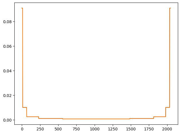
Note that elements of $\Pi$ depend only on the number of features in the data and thus can be pre-computed. Plot of the diagonal elements of $\Pi$ for the wine dataset with 11 features is shown below. In this case, $\Pi$ is a $2^{11} \times 2^{11}$ = $2048 \times 2048$ diagonal matrix. As noted above, the first and last values are $\infty$ , and thus the plot below excludes those values. The plot shows a broad trough with large values on either side. This is because the first and last few coalitions examine the features in relative isolation. The first few coalitions contain mostly zeros and a few ones, and thus consider the effect of the presence of the features corresponding to the ones whereas the last few coalitions contain mostly ones and a few zeros and thus consider the effect of the absence of the features corresponding to the zeros. Such coalitions are more discriminating in evaluating the importance of those features and are given higher weight. For a formal proof of 4 , refer to the supplementary material of the original paper.

Before we proceed further, let’s consider a simple example to illustrate these ideas. Let’s consider the wine dataset. As shown in the screenshot below, this dataset has 11 predictor variables and 1 target variable (quality).

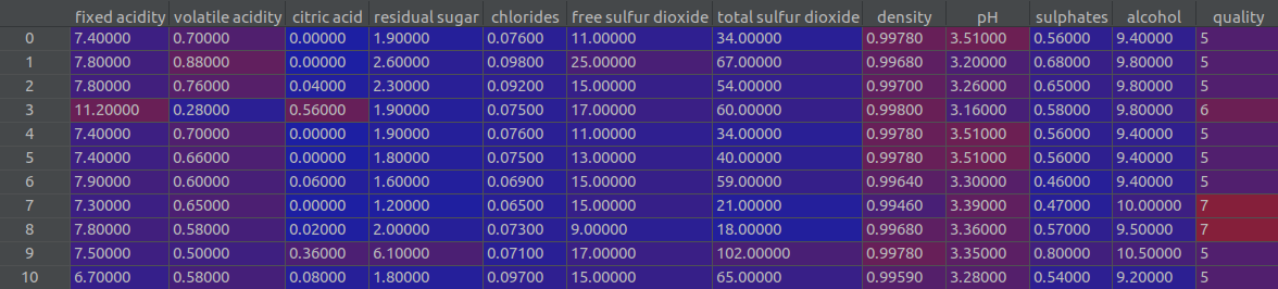
For simplicity let’s assume our training dataset consists of just the first three predictor variables (fixed acidity, volatile acidity, citric acid) and the 10 rows shown in the figure above. We already have a model trained on this training dataset, and we wish to explain the model’s prediction on row #3: fixed acidity = 11.2, volatile acidity = 0.28 and citric acid = 0.56

Consider first the case of $\lvert c_i \rvert = 0$ . This corresponds to the case when all feature values are turned off (for all $i$ from 1 to M, $z_i^\prime = 0$ ) and therefore $g(z^\prime)=\Phi_0$ (from 2). In the original paper, this is called the “missingness” constraint. Since $\pi(z^\prime)$ for this case = $\infty$ (from 4), this enforces (from 1)

$g(z^\prime) = f(h(z^\prime))$

$f(h(z^\prime))$ in this case is simply the average of the model prediction over the training dataset. Let’s call this $E(f)$ , meaning the expectation of the model prediction $f$ over all training instances.

Now let’s consider the case $\lvert c_i \rvert = M$ , the number of features. This corresponds to the case where all feature values are turned on (all $z_i^\prime = 1$ ) and therefore

$g(z^\prime)=\Phi_0 + \Sigma_{i=1}^{M}\Phi_i$

Again, since $\pi(z^\prime)$ for this case = $\infty$ (from 4), this enforces (from 1)

$g(z^\prime) = f(h(z^\prime))$

$f(h(z^\prime))$ in this case is the model prediction for the specific data instance $x$ for which we want to explain the model’s prediction ( $h(z^\prime) = x$ ). In other words,

(5) $\begin{equation*} \Phi_0 + \Sigma_{i=1}^{M}\Phi_i = f(x) \end{equation*}$

So the upshot is that our definition of $\Pi$ fixes the first shapley value $\Phi_0$ and imposes a constraint on the other values ( 5)

Let’s consider the case of $\lvert c_i \rvert = 2$ . Since the total number of features is 3 (remember we are only considering the first three features), we can easily enumerate all possible combination of features. The feature permutation matrix $C$ ( $8\times3$ ) looks like this:

$C=\begin{bmatrix} 1& 0 & 0 & 0 \\ 1& 1 & 0 & 0 \\ 1& 0 & 1 & 0 \\ 1& 0 & 0 & 1 \\ 1& 0 & 1 & 1 \\ 1& 1 & 1 & 0 \\ 1& 1 & 0 & 1 \\ 1& 1 & 1 & 1 \\ \end{bmatrix}$

The first row corresponds to the “base case” when all features are missing and the last row corresponds to the case when all feature values are set to the data instance features $x$ for which shapley values are being calculated. Rows 5, 6 and 7 correspond to the case when 2 features are present and the third is missing (row 5 corresponds to the case where the first feature is missing, row 6 the case where the third feature is missing and row 7 the case where the second feature is missing). Using 4 we can easily calculate the value of elements $\Pi$ :

$\pi_2 = \frac{2}{\binom{3}{2} \times 2 \times 1} = 0.33$

How do we calculate $f(h(z^\prime))$ when some features are missing? There are multiple ways to do this – one way is to randomly pick values for the missing features from the training dataset, another is to consider all possible values for the missing features that occur in the training data (full training data or a summarized version of it) and average the model predictions. For example, let’s say your training data consists of $T$ instances. You replace the values of the features for which $z^\prime = 1$ , i.e., the “present” or “non-missing” features with the corresponding coalition feature values (and leave the other feature features unchanged) for all $T$ instances, and then average out the model predictions. This requires running the model predict function $T$ times, but doesn’t require any knowledge of the model’s internal structure. The model could be a linear/logistic regression model, Gradient Boosted Tree, Neural Network..

So now that we have fixed the value of $\Phi_0$ , and established a constraint on the other Shapley values (5), we need to use the constraint to eliminate one Shapley value in 3. Let’s pick the last Shapley value, $\Phi_M$ .

From 5,

(6) $\begin{equation*} \begin{aligned} \Phi_M &= f(x) - \Phi_0 - \Phi_1 \cdots -\Phi_{M-1} \\ &= f(x) - E(f) -\Phi_1 \cdots -\Phi_{M-1} \end{aligned} \end{equation*}$

Let’s now consider the term inside the norm in 3. This term is a column vector of dimension $N\times 1$ , with element indices ranging from $0\leq i \leq N-1$ . This column vector is a difference of model evaluations on the various feature combinations and the matrix vector product of the coalition matrix and the Shapley values. The first and the last elements of this column vector must be 0 because they correspond to the two constrains we discussed above. For ease of notation, let’s denote the remaining model evaluations as $f_1, f_2, \cdots, f_{N-2}$ . Also, let $C_{ij}$ be the $i,j$ element of the coalition matrix. Writing out the non-zero elements of the column vector, we get:

(7) $\begin{equation*} \begin{aligned} f(h(z^\prime)) - C\Phi &= \begin{bmatrix} f_1 - C_{10}\Phi_0 - C_{11}\Phi_1 - C_{12}\Phi_2 - \cdots - C_{1M}\Phi_M \\ f_2 - C_{20}\Phi_0 - C_{21}\Phi_1 - C_{22}\Phi_2 - \cdots - C_{2M}\Phi_M \\ \vdots \\ f_{N-2} - C_{N-2,0}\Phi_0 - C_{N-2,1}\Phi_1 - C_{N-2,2}\Phi_2 - \cdots - C_{N-2,M}\Phi_M \end{bmatrix}\\ &= \begin{bmatrix} f_1 - \Phi_0 - C_{1M}(f(x) - \Phi_0 - \Phi_1 \cdots -\Phi_{M-1}) - C_{11}\Phi_1 - C_{12}\Phi_2 - \cdots - C_{1,M-1}\Phi_{M-1} \\ f_2 - \Phi_0 - C_{2M}(f(x) - \Phi_0 - \Phi_1 \cdots -\Phi_{M-1}) - C_{21}\Phi_1 - C_{22}\Phi_2 - \cdots - C_{2,M-1}\Phi_{M-1} \\ \vdots \\ f_{N-2} - \Phi_0 - C_{N-2,M}(f(x) - \Phi_0 - \Phi_1 \cdots -\Phi_{M-1}) - C_{N-2,1}\Phi_1 - C_{N-2,2}\Phi_2 - \cdots - C_{N-2,M-1}\Phi_{M-1} \end{bmatrix} \\ \text{because the first column of the coalition matrix consists of ones}\\ &= \begin{bmatrix} f_1 - \Phi_0 - C_{1M}(f(x) - \Phi_0) - (C_{11} - C_{1M})\Phi_1 - (C_{12} - C_{1M})\Phi_2 - \cdots - (C_{1,M-1} - C_{1M})\Phi_{M-1} \\ f_2 - \Phi_0 - C_{2M}(f(x) - \Phi_0) - (C_{21} - C_{2M})\Phi_1 - (C_{22} - C_{2M})\Phi_2 - \cdots - (C_{2,M-1}-C_{2M})\Phi_{M-1} \\ \vdots \\ f_{N-2} - \Phi_0 - C_{N-2,M}(f(x) - \Phi_0) - (C_{N-2,1}-C_{N-2,M})\Phi_1 - (C_{N-2,2}-C_{N-2,M})\Phi_2 - \cdots - (C_{N-2,M-1}--C_{N-2,M)\Phi_{M-1} \end{bmatrix} \end{aligned} \end{equation*}$

Denoting column $i$ of the coalition matrix by $C_i$ and defining

(8) $\begin{equation*} f^*= \begin{bmatrix} f_1 - \Phi_0 - C_{1M}(f(x) - \Phi_0)\\ f_2 - \Phi_0 - C_{2M}(f(x) - \Phi_0) \\ \vdots \\ f_{N-2} - \Phi_0 - C_{N-2,M}(f(x) - \Phi_0) \end{bmatrix} \end{equation*}$

and

(9) $\begin{equation*} C^*= \begin{bmatrix} C_1-C_M, C_2-C_M \cdots C_{M-1}-C_M \end{bmatrix} \end{equation*}$

The minimization in 3 is equivalent to minimizing:

(10) $\begin{equation*} {\lVert f^*- C^*\Phi \rVert}^2 \Pi \end{equation*}$

$C^*$ is a $N-2 \times M-1$ matrix, $f^*$ is a $N-2 \times 1$ vector, $\Phi$ is a $M-1 \times 1$ vector of shapley values and $\Pi$ is a $N-2 \times N-2$ diagonal matrix. This is an overdetermined system of equations whose least squares solution is given by solving:

$C^*^TC\Pi\Phi=C^*^T\Pi f(h(z^\prime))$

For the Python implementation, see function _shap in my Kernel SHAP implementation.

Telesens

Be the first to comment

Leave a Reply Cancel reply