

In this post, I’ll describe some experiments on word2vec, a technique invented by researchers at Google (1310.4546">https://arxiv.org/abs/1310.4546">1310.4546) that aims to find compact vector representations for words in a natural language that capture natural semantic relationships between words. For example, vec(“Madrid”) – vec(“Spain”) should be close to vec(“Paris”) – vec(“France”). I refer you to the original paper for a detailed problem description and the network architecture of the neural network used to train the word vectors.
In my investigation, I wanted to examine if it is possible to take word vectors trained from a larger corpus to initialize the embedding matrices for training on a smaller, more context specific corpus. This issue arises in many real world applications where one has a moderate amount of context specific data. This data may not be large enough to train word vectors from scratch. It would be nice if one could start with the word vectors trained on a larger corpus and use the context specific information in the smaller corpus to tweak the pre-trained word vectors so that they reflect the knowledge embedded in the context specific corpus without losing the relationships learnt from training on the more general corpus.
During this investigation, I also learnt a great deal about pre-processing the text in the training corpus, the details of building a batch consisting of a target word, in-context words and out-of-context words that is used to run the forward pass and compute loss and methods used to visualize the trained word vectors. I’ll describe some of these insights in this post which may be useful for other practitioners.
Organization
The post is organized as follows:
- Section 1 describes the python code base that I used as the starting point for my implementation and the reasons for making that choice
- Section 2 covers the text pre-processing steps which can significantly impact the quality of the resulting word vectors
- Section 3 looks at the motivation and implementation details for some of the innovations introduced by in word2vec such as frequent word sub-sampling and negative word sampling
- Section 4 describes the process for creating a batch that is used to run the forward pass and compute loss
- Section 5 shows how to visualizing embedding vectors by converting them into a low dimensional space using t-SNE and PCA and the relative merits of each technique
- Section 6 describes the results of using a pre-trained word2vec model to initialize the embedding matrix for training on new data
Table of Contents
1. Python Code Base
There are many open source code libraries available on the web under open source MIT/BSD style licenses that implement word2vec. The original Google word2vec code and the gensim library (https://radimrehurek.com/gensim/) are two popular choices. The gensim library implements many other document and topic modeling techniques such as doc2vec and LDA was well. Since I’m new to topic modeling, I wanted to use a relatively simple implementation that was easy to understand and focused on the essential elements of the word2vec algorithm without the extra code to implement features that I didn’t need. Furthermore, the gensim library is pure python and doesn’t use a machine learning frameword such as PyTorch. This means that much of the boilerplate calculations in machine learning such as calculating gradients and updating parameters has to be implemented from scratch, adding additional complexity.
After some web search, I settled on the implementation in this repo: https://github.com/fanglanting/skip-gram-pytorch. This code uses the PyTorch machine learning library that is available on Linux and Windows and implements the skip-gram model as described in the original word2vec paper without any additional complexity.
Text Corpus
There are two important considerations in choosing a text corpus.
- Since I wanted to investigate the feasibility of using word vectors trained from a larger corpus to initialize the embedding matrix for a smaller, more context specific corpus, I needed two corpuses – a larger and more general corpus and a smaller, context specific corpus
- Each corpus needs to be small enough that I could train it on my home deep learning machine (equipped with a single NVIDIA 1080Ti GPU) in a reasonable amount of time
I looked into using word embedding models trained on the Google News database and the GloVe model (https://nlp.stanford.edu/projects/glove/) provided by Google and Stanford respectively, but these models only contain the part of the embedding matrix that is needed for inference, not the part required for training. I’ll elaborate on this issue in more detail later.
The solution I ended up using was abstracts from the Arxiv database. Using a python scrapper, I downloaded all abstracts in the “cs” (computer science) category from 2010-2017. This resulted in about 125000 files containing ~122 MB of data and constituted the larger, more general corpus. I further downloaded all abstracts in stats.ML (Machine Learning subcategory of Statistics) that contain the word “learning” from 2013-2017. This resulted in about 10500 files containing ~11 MB of data and constituted the smaller, more context specific corpus. I then ran the word2vec algorithm as implemented by fanglanting (with some modifications, described below) on this data.
2. Text Pre-Processing
The main goal of text pre-processing is to remove redundant words that may enhance readability but doesn’t provide additional context that word2vec training can capture. Pre-processing also keeps the vocabulary from becoming unnecessarily large. For example, a word in upper case is identical to that word in lower case but would be represented as a separate word in the vocabulary unless appropriate case conversion is performed. A smaller vocabulary means a less difficult training task and also results in a smaller word2vec model since each word is a row in the embedding matrices. Thus it makes sense to try to keep the size of the vocabulary down by eliminating redundant words. Shown below is a list of pre-processing steps I used in my experiment.
- Convert all links/urls (text containing “http” or “www”) to the token LINK
- Convert all latex expressions (text containing “$”) to LATEX
- Ignore all numbers and text containing numbers
- Convert all letters to lower case
- Removed all punctuation marks (word. becomes word, hello! becomes hello)
- I considered eliminating compound words, misspellings and author names in the text by using an English dictionary and only retaining valid English words. “Enchant” is a popular dictionary with Python bindings that is commonly used for this task, however it turned out that a x64, Win 10 version of “Enchant” is not available. While the failure to remove these spurious words leads to unnecessary growth in the word vocabulary, they may not have a significant impact on the quality of the word vectors as the spurious words are unlikely to be very frequent. For example, the same spelling mistake is unlikely to be repeated more than once. It is interesting to note that in the arxiv data, there are numerous instances where the white space between two successive words is missing. Since I use white space as the delimiter to tokenize the text, the missing white space leads to the two words being added to the vocabulary as a combined word. For example, consider some example text from abstract #1412.2632:
The task of reconstructing a matrix given a sample of observedentries is known as the matrix completion problem. it arises ina wide range of problems, including recommender systems, collaborativefiltering, dimensionality reduction, image processing, quantum physics or multi-class classificationto name a few. most works have focused on recovering an unknown real-valued low-rankmatrix from randomly sub-sampling its entries.here, we investigate the case where the observations take a finite number of values, corresponding for examples to ratings in recommender systems or labels in multi-class classification.
- I experimented with two other popular text processing techniques – stop word removal and stemming. Stop word removal involves removing words such as “the”, “and”, “but” that provide little contextual information. Stemming involves removing the word endings such that a word is reduced to its “core”. The core may or may not be a valid word. For example, “intuition”, “intuitive”, “intuitively” would all be reduced to “intuit”. Stemming can be effective on small corpuses as it increases the frequency of related but distinct words. I did not notice an appreciable change in the quality of the word vectors with or without these techniques. For stop word removal, this could be because frequent word sub-sampling (described later) keeps many of the stop words from being included in training batches.
3. Text Sub-Sampling Techniques
Creating a Word Vocabulary
After reading the text corpus and applying the text processing techniques mentioned in the previous section, we obtain a “bag of words” that maintain the word order in the original documents. The next task is to create a word vocabulary from this bag of words. A word vocabulary consists of a mapping between words and their unique numeric indices. The indices are used to look up the embedding vector corresponding to a word.
To create the word vocabulary, we first rank the words in the order of frequency and create a table that maps each word to its index in the frequency table. Each word in the corpus is then replaced by its index. This process is shown below for one abstract.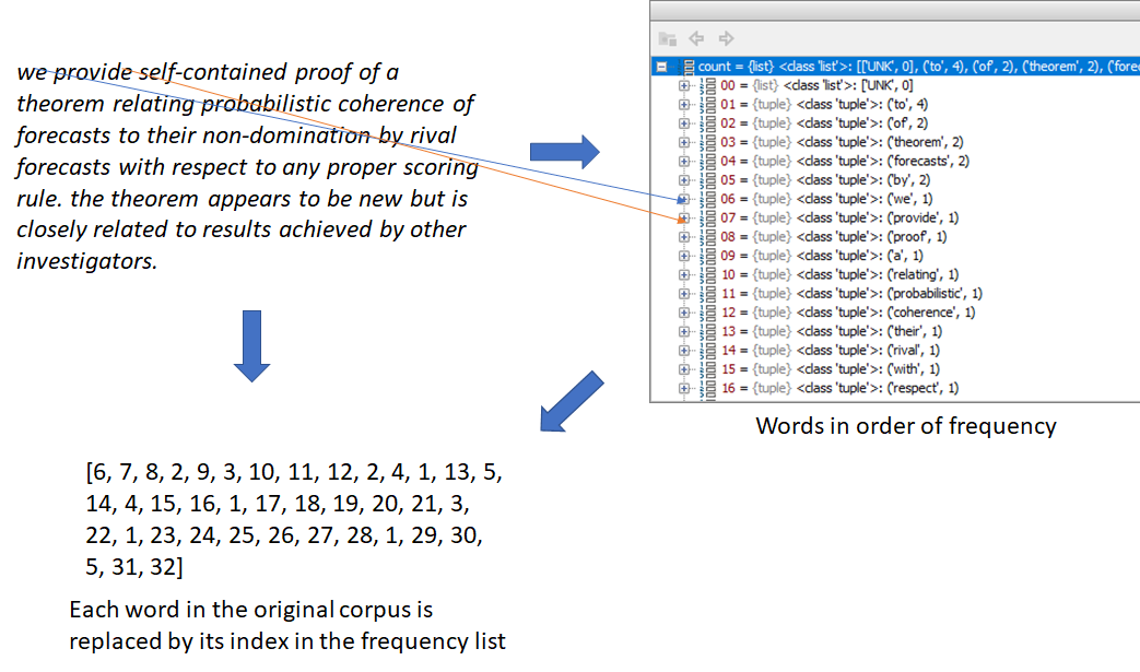 The word vocabulary is constructed from the frequency table. The word frequency table maps indices to words (1:
“to”, 2: “of”, 3: “theorem” and so on). The inverse of the word frequencies, i.e., a table that maps words to corresponding indices is also maintained. It is possible to select a smaller vocabulary size than the total number of unique words in a corpus. In this case, the top n (n = specified vocabulary size) words from the frequency table are selected to be included in the vocabulary. While replacing each word in the corpus with its index, words that don’t appear in the vocabulary are dropped.
Frequent Word Sub-Sampling
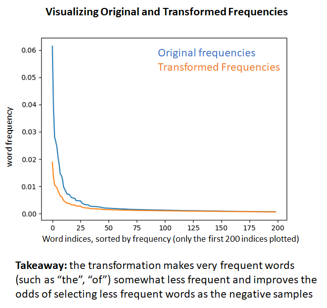
Next, we sub-sample more frequent words by applying an inverse function to the word frequencies that has a higher value for lower frequency words. The intuition is that we want to retain lower frequency words as they are more meaningful than higher frequency words that are likely to be grammar constructs. This process is shown in the figures below. Also refer to http://mccormickml.com/2017/01/11/word2vec-tutorial-part-2-negative-sampling/ for a good explanation of this sub-sampling technique. According to this post, the sub-sampling function used in the C implementation of word2vec provided by Google differs from the one mentioned in their paper.
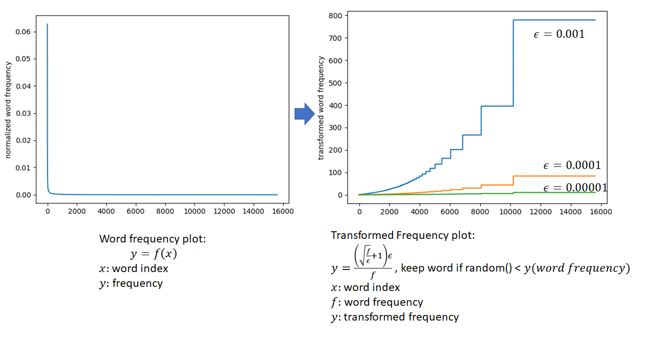
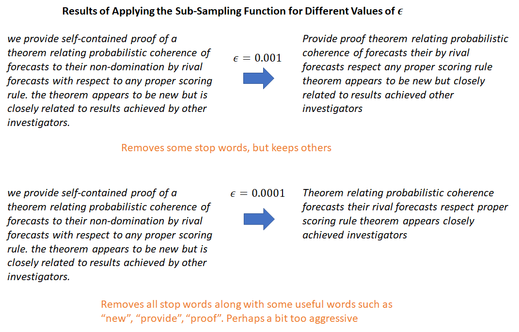
after applying frequent word sub-sampling, we have converted the original word corpus into a list of indices where some words that failed the sub-sampling test don’t appear. Since the sub-sampling is applied stochastically (notice the use of random() in the figure above), a given word is never entirely “banned” from the corpus, it may be included or excluded depending on chance and its frequency. The lower the frequency, the more likely it is to be included. Also, as a result of the sub-sampling, the total size of the corpus is less than the original corpus, helping to speed up training.
Negative Word Sampling
In this step, we create a special sampling array to be used for negative word sampling (refer to the word2vec paper if you don’t know what this means). The word2vec authors propose applying a transformation to the word frequencies and selecting the negative samples according to the probability distribution induced by these transformed frequencies. To make this easier to understand, I’ll use a simple example where our vocabulary consists of just 4 words – “the”, “of”, ” machine”, and “learning”.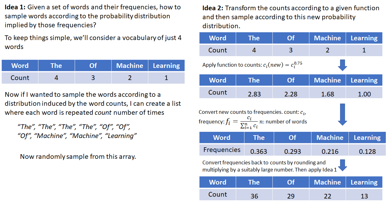
4. Creating a Batch
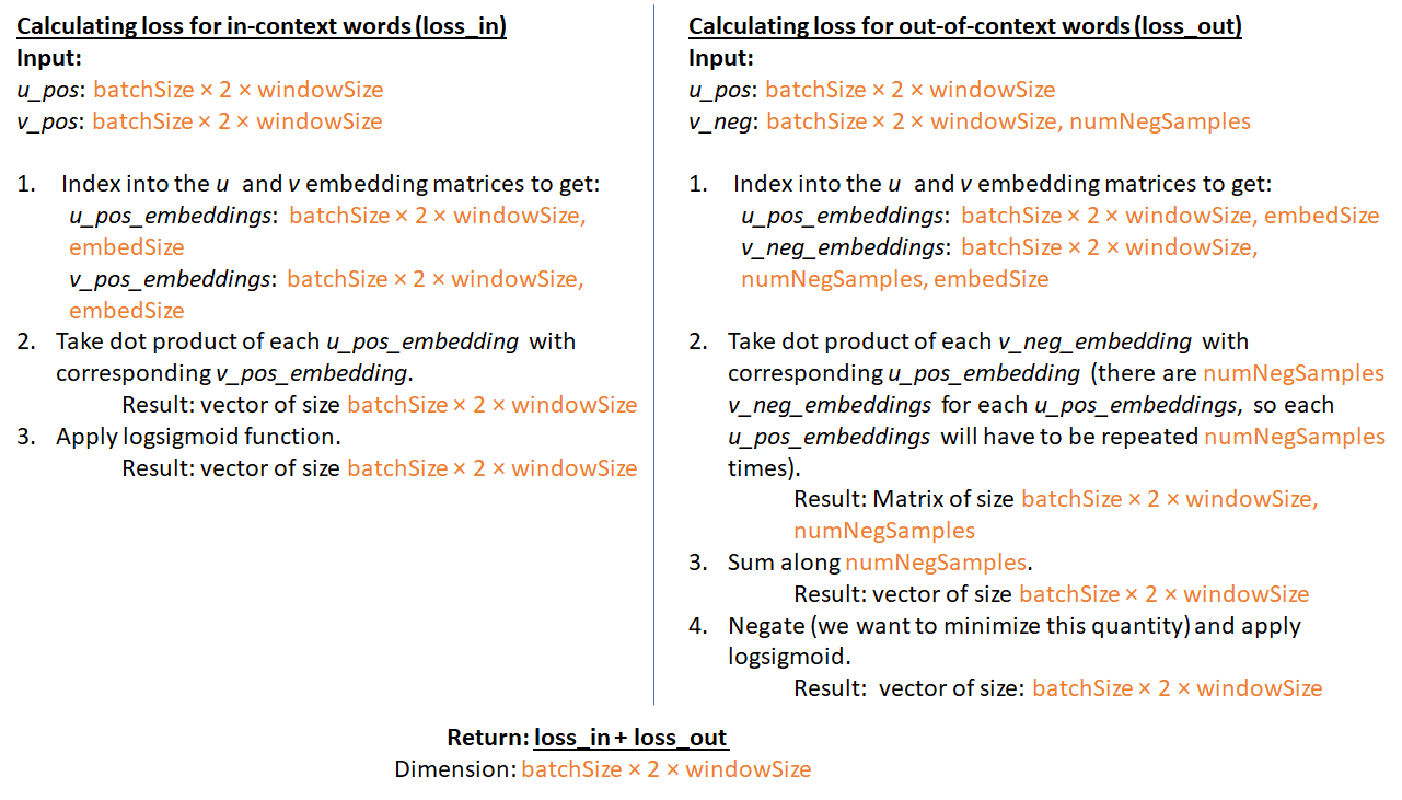
For better hardware utilization, machine learning algorithms operate on a batch of data instead of a single unit of data at a time. The figures below show how a batch is created for training a word2vec model and how the “loss” (objective function to be minimized) is calculated.
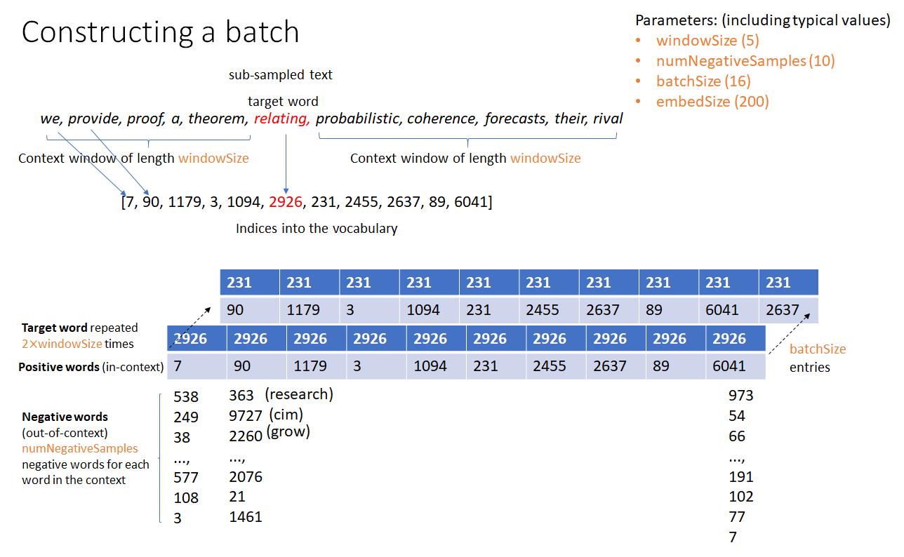
Note that sliding windows (consisting of the target word and in-context words) can be chosen in many ways – the pointer to the target word can moved to the next word in the corpus or a random word in the corpus can be chosen as the next target word. In my current implementation, the first method is used. The second method may produce better results as it is more stochastic in nature.
Once we have a loss function, standard gradient descent is used to compute gradients and update the embedding vectors in order to minimize the loss. This functionality is provided out of the box by deep learning libraries.
Training Performance
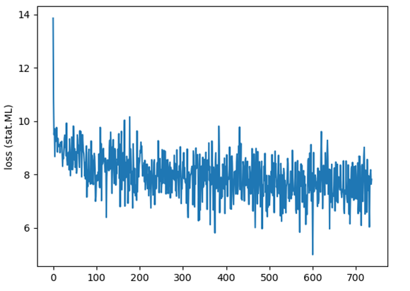
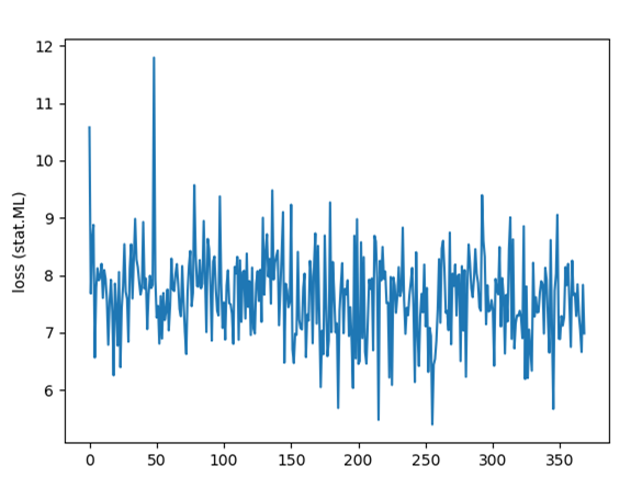
Training on the stat.ML dataset for 10 epochs took about an hour and on the cs dataset for 10 epochs about 4 hours on my Windows 10 machine with a NVIDIA 1080Ti GPU. The loss declines rapidly at first and then hovers around 7.5. I used the standard SGD (Stochastic Gradient Descent) optimizer with a constant learning rate. Here’s the progression of the loss function for the stat.ML dataset:
Using the Word2Vec Models
So once you have trained the word2vec models, what can they be used for? One of the things you can do with word vectors is to determine similar words. The whole idea behind word2vec is to determine a lower dimensional representation for words where similar words appear closer to each other. So, to determine similar words to a target word, one simply needs to calculate the dot product of the embedding vector corresponding to the target word (called target embedding vector from now on) with the other embedding vectors and rank the words in order of dot product. The procedure is as follows:
- Load the model and the vocabulary. Inspecting the loaded model in a python debugger in my pytorch implementation, I see the following:
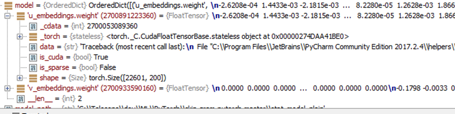
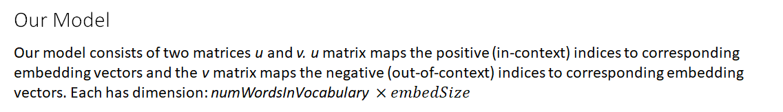
there are two matrices u_embeddings and v_embeddings, corresponding to the u and v matrices mentioned above. Only the u_embedding matrix is needed for inference. The size of the matrix is numWordsInVocabulary
 embedSize.
 - Given a target word, we look up the index of this word from the vocabulary. Then, we look up the corresponding embedding vector from the embedding matrix. To determine similar words, we calculate the dot product of the embedding vectors corresponding to other words in the vocabulary with the target embedding vector and sort the dot products from high to low.
Let’s look at the top 9 closest words for target words “embeddings”, “learning”, “optimization” and “loss”
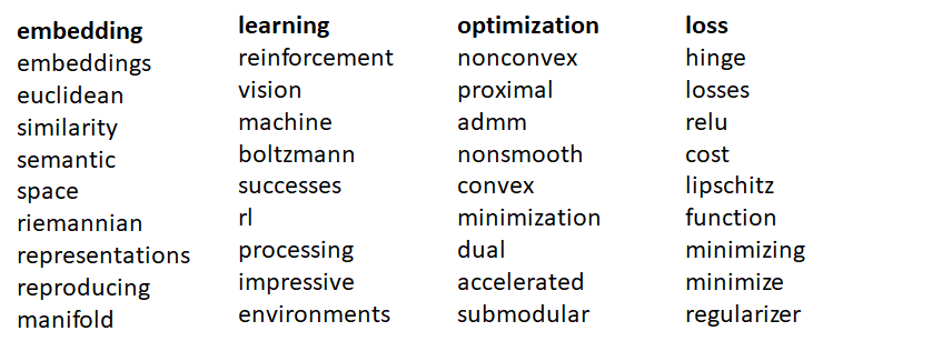
The top 9 words for each target word are expected to occur in the same context as the target word, so our model appears to have learnt the word relationships.
5. Visualizing the Word Embeddings
It would be nice to visually see which words are close to a target word. This can not be done in the original embedding space as the dimension of the embedding vector is usually quite high (in the hundreds). We need some method to reduce the dimensionality of the embeddings so that the vectors can be represented as a 2 or 3 dimensional vector (which can be plotted in 2D or 3D) while losing as little information in the original vector as possible.
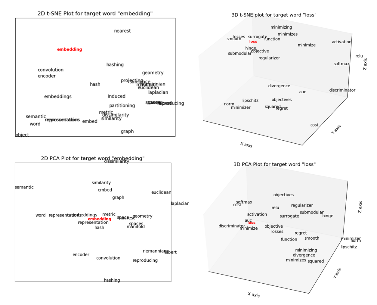
Two common methods used for representing high dimensional data in lower dimensions are Principle Component Analysis (PCA) and t-SNE (Stochastic Neighbor Embedding using a Student t-distribution). The figures below show the 2D and 3D vectors generated by PCA and t-SNE for the top 25 words for target words “loss” and “embedding”.
Quick Primer: t-SNE and PCA
t-SNE tries to minimize a single Kullback-Leibler divergence between a joint probability distribution,  , in the high-dimensional space and a joint probability distribution,
  , in the low-dimensional space:

Here  is the conditional probability that
  would pick
  as its neighbor if neighbors were picked in proportion to their probability density under a student-t distribution centered at . For more details refer to the original paper http://www.jmlr.org/papers/volume9/vandermaaten08a/vandermaaten08a.pdf
The important point to understand about t-SNE is that it is mainly a visualization technique to visualize high-dimensional data by giving each datapoint a location in a two or three-dimensional map. t-SNE aims to solve a problem known as the crowding problem, which is that somewhat similar points in higher dimension tend to collapse on top of each other in lower dimensions. t-SNE aims to preserve the local structure of the high-dimensional data while also revealing global structure such as the presence of clusters at several scales.
PCA is a general dimensionality reduction technique that involves finding a set of basis vectors and projecting the higher dimensional data on these basis vectors such that the data can now be represented using fewer dimensions preserving as much variation in the data as possible. The intuition being that in many cases, the higher dimensional data has most of its variation along only a few axes and little information is lost by discarding the other axes. PCA performs this dimensionality reduction in a mathematically rigorous manner, producing scores for how much variation in the original data is captured along each axis. PCA has three outputs:
- Variance in the original data captured along each dimension of the output basis vectors (also called “principal vectors” or “principal components”). PCA also tells us how much “information” is lost by discarding the other dimensions.
- The direction of the principal vectors (in the vector space of the original data)
- The data points re-projected along the principal vectors
The figure below shows an application of PCA in two dimensions. The blue dots are randomly generated points in an ellipse with major axis = 10 and minor axis = 3. The points are rotated by about 60 degrees. One can see that most of the variation in this data is along the major axis of the ellipse. The red dots show the re-projections of 20 randomly selected points after performing a PCA with number of components equal to 1. The black line shows the direction of the principal component vector. PCA tells us that about 92% of the variation in this data is captured by projecting it in one dimension. If the data were less elliptical, the variance captured by projecting along along one dimension would be smaller. PCA captures this information in a mathematically rigorous way.
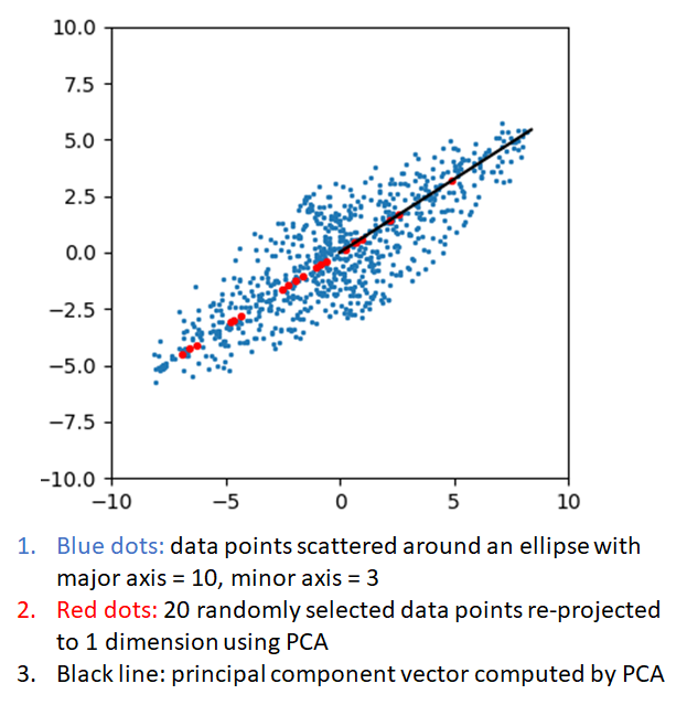
Now, the original 2 dimensional data can be represented by an equal number of 1 dimensional points along the principal vector, with little loss of information.
For more information, see the wikipedia article about PCA (https://en.wikipedia.org/wiki/Principal_component_analysis).
The example shown above doesn’t confer any visualization benefit as we can visualize both the original 2 dimensional data and the 1 dimensional data after applying PCA. However it is easy to see how PCA can be used to visualize higher dimensional data by reprojecting it along 2 or 3 dimensions. The larger the variation that is captured along the lower dimensions, the more accurate will be the resulting visualization.
Which is Better: PCA or t-SNE?
As I mentioned earlier, t-SNE is a visualization technique designed to represent high dimensional data in 2 or 3 dimensions, not a dimensionality reduction technique. PCA is a general dimensionality reduction technique that may also result in good visualizations. As such, the two are designed for different purposes and are not directly comparable. However, I still could’t resist doing a comparison.
Since t-SNE and PCA work using entirely definitely mathematical principles, there is no obvious way to rigorously compare the two. One could visually look at the top-n word vectors in 2 or 3 dimensions produced by each technique (as shown in the pictures above), however it is hard to say which one is better. I came up with the following methodology. Suppose, for a certain target word, we rank the top 50 words (from high to low) according to the dot product of their embedding vectors with the target embedding vector. The top word in this list is the closest match and the last word the worst match to the target word. This list uses the full embedding vectors and is therefore the best we can do. Let’s call this list  , “gs” means “gold standard”. Now lets use t-SNE and PCA to generate a lower dimensional representations of the 50 words and rank the words by the dot products calculated in the lower dimensional space. We call the rankings generated by t-SNE and PCA
  and
and  respectively.
Let’s look at the first 5 words ranked according to the dot products computed using the original embeddings and the lower dimensional representations for the target word “embedding”
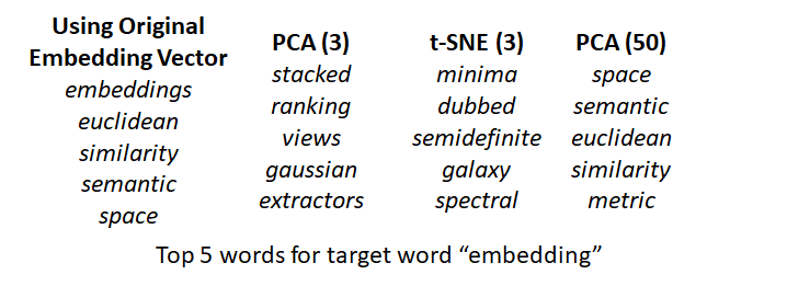
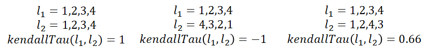
We can see that the number of dimensions of the lower dimensional space makes a big difference in the quality of the ranking. Using dimension 3 (the highest dimension that we can visualize), the top 5 words don’t appear to be in the same context as the target word “embedding” at all. Using a 50 dimensional representation, the top 5 results start to look a lot better. We can formalize this idea by asking the question – “how similar are and to the gold standard list “? These lists contain the same words, but in different order. The question can be answered using a metric called the Kendall tau rank distance that counts the number of pairwise disagreements between two ranked lists. The larger the distance, the more dissimilar the two lists. The kendall tau distance varies between 1 for identical lists to -1 for lists that are reverse of each other.
Using the kendallTau distance, we can compare how close the ranking generated by dot products computed from t-SNE and PCA are to the gold standard ranking. The results are shown below for target words “Embedding”, “Learning”, “Optimization” and “Loss”
| Words/Kendall Tau Score | PCA | t-SNE |
| Embedding | -0.17 | -0.33 |
| Learning | 0.12 | 0.103 |
| Optimization | 0.23 | -0.26 |
| Loss | 0.20 | -0.22 |
It appears that PCA produces a ranking that is closer to the gold standard ranking than t-SNE does.
To reiterate, this doesn’t mean that PCA is “better” than t-SNE. This result simply appears to suggest that PCA is better at creating a lower dimensional representation that preserves the discriminating power of the embedding vectors. t-SNE may still result in better visualizations of the lower dimensional data, which it is designed to do.
Common sense suggests that as we add more dimensions to our lower dimensional representation, the kendall-tau score should improve. In fact, since PCA gives us the total variance captured as a percentage, we can plot the total variance captured and the kendall-tau score against the number of dimensions. The two quantities are on a similar scale (-1 to +1 for kendall-tau and 0-1 for total variance captured) and can thus be plotted on the same graph.
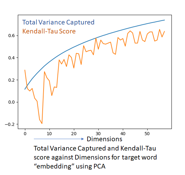
The kendall-tau score is a lot noisier, but follows the total variance captured (which by definition is a smoothly increasing function, as adding an extra dimension can’t result in a loss of information) as the number of dimensions is increased. Another interesting observation is that the variance of the embedding vectors appears to be well distributed among the available dimensions. A 50 dimensional representation is able to capture about 65% of the variation in the data, which is good but also suggests that the dimensionality of the embedding vectors can’t be significantly reduced without an accompanying reduced in discriminating power.
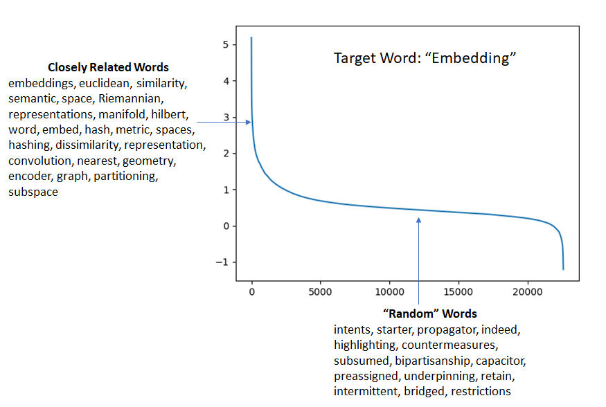
Variation of the Embedding Vector dot-product
Intuition suggests that for a given target word, there are a few words that are closely related and expected to occur more frequently in the same context as the target word – for example, we expect the word “embedding” to be accompanied by “word”, “representation”, “subspace” and so on. In contrast, the vast majority of the words in the vocabulary will occur in the same context as the target word largely by chance, without a strong preference for one word over the other. This intuition is supported by the variation of the dot product of the target embedding vector and other embedding vectors. This dot product is high for a handful of words and then falls rapidly and gently declines for the remaining words.
6. Using Pre-Trained Models to Bootstrap Training on Smaller Corpuses
In this section, we’ll examine if it is possible to take a word2vec model trained on a large, more general corpus and use the trained model to initialize the embedding matrices for a model that will be trained from a smaller, more topic specific corpus. This use case arises when a relatively small amount of topic specific data is available; this data has enough context information for the limited number of topic specific words but perhaps not enough context examples for the much larger number of general words. The intuition is that the model can start from the general embeddings trained on the larger, more general corpus while benefiting from the additional fine-tuning provided by training on the topic sensitive corpus.
To test this idea, I used a python scrapper script to download all arxiv abstracts from the “CS” (computer science) category from 2010-2017. This resulted in about 125000 files adding up to ~122MB of data. This constituted the large corpus. For the smaller corpus, I downloaded abstracts in the stat.ML subcategory that contained the word “learning”. This resulted in 10447 files, 10.6 MB of data.
I then trained three separate models:
Model 1: Trained on the stat.ML dataset
Model 2: Trained on the cs dataset
Model 3: Trained on the stat.ML dataset, but initialized using Model 2.
Note that training Model 3 is not simply a matter of using the u and v matrices from Model 2. One must ensure that during frequent word sub-sampling and sampling of negative words, the word frequencies from the current corpus are used but while creating the batch that will be used to run the forward pass and computing loss, the indices into the original vocabulary are used. I also made a simplifying assumption that the smaller vocabulary is completely contained within the larger vocabulary. This is to keep the implementation simple. The assumption can be removed by adding rows in the embedding matrix for words not found in the larger corpus and randomly initializing the elements (as they would be initialized if a pre-trained model was not used)
Results
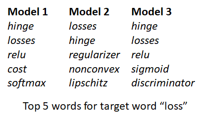
We can see that some of the machine learning related words such as “relu” and “sigmoid” made it back in the top 5 using Model 3.
The figure below shows the progression of the loss function. We don’t see the sharp drop in the beginning that we saw earlier when the model was trained from scratch. This makes sense as we are starting from a good point already.
There are a few additional points that one can verify. The embedding vectors corresponding to words that are in the CS vocabulary but not in the stats.ML vocabulary shouldn’t be modified by training on stats.ML. This was verified by looking at the those vectors before and after the training.
Additionally, the magnitude of the difference vector, i.e., an embedding vector after training minus that vector prior to training, should be higher for words that are more relevant to stats.ML than for general words that are not salient to stats.ML. This also appears to be the case. Shown below are few words that are near the top and bottom respectively when ranked by the magnitude of the difference vector
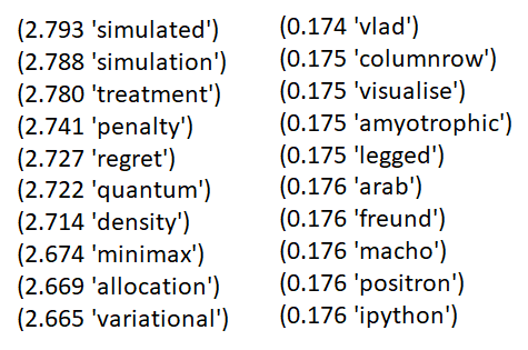
The words in the list on the left are much more relevant to stats.ML than words in the list on the right.
Conclusion
The results of this experiment suggest that using a pre-trained model to initialize the embedding matrices is feasible and may provide some benefits over starting from random initialization of the embedding matrices. However more work is needed to quantify how much of the context specific information can be captured by using pre-trained embeddings and how much training needs to be performed. It may be that if one trains on the new data for long enough, the “general” information present in the original embeddings may get lost which will defeat the point of using the pre-trained embeddings.
Leave a Reply