

The purpose of this post is to discuss my current understanding of roofline charts. Let me lay some background first. Before I got into machine learning, I knew little about computer architecture. My knowledge mostly consisted of a high level understanding of processor speed, RAM, some knowledge about cache’s etc. When comparing two processors, I would look at the clock speed, and assume that the faster processor is necessarily better. Now after dealing with Deep Learning SW and HW for a while, my understanding of computer architecture is more nuanced.
For a long time, there were two types of processors that dominated computers – CPUs and GPUs. This is no longer the case. The tremendous success of deep learning models in image analysis, speech processing, document analysis etc., have led to a surge of interest in designing specialized hardware optimized to accelerate training deep learning models and running data through these models (called “inference”) both on the “edge” (inference on embedded devices) and on the cloud. So much so that The Economist recently published an article titled “Artificial intelligence is awakening the chip industry’s animal spirits” about the exploding market in chips designed for deep learning (and more broadly speaking, for AI), this market is expected to reach 30B by 2022. One reason for this resurgence of interest is that deep learning models are almost a hardware architect’s dream – they are deterministic, sequential and massively parallel. If that wasn’t enough, deep learning calculations don’t require high precision and can be easily carried out using small data types such as 4-8 bit integers.
In the last couple of years, there has been a Cambrian explosion of specialized hardware from both big companies (TPUs from Google, project Brainwave from Microsoft, ACAP from Xilinx) as well as startups such as Graphcore, Mythic, Cerebrus and many others. With so many options for deep learning HW, the question arises – how does one compare the performance of various deep learning algorithms on these hardware in an insightful way? Roofline charts are one way to do this. In the remainder of the post, I’ll first briefly describe why GPUs are highly effective deep learning processors, this will naturally lead to the concepts of “OPS” or “FLOPS” (Operations per Second or Floating Point Operatios per Second when the operations are floating point) and “AI” (Arithmetic Intensity) which are the quantities plotted in a roofline chart. Then we’ll look at at a couple of examples related to various types of memories on a GPU and the roofline chart shown in Google’s white paper about TPUs.
Why are GPUs so Effective in Deep Learning?
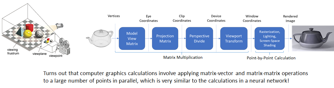
GPUs are highly parallel processors – they consist of thousands of “streaming microprocessors” designed to carry out arithmetic operations on large volumes of data in parallel. GPU’s being Graphics Processing Units were designed to accelerate computer graphics calculations, not for deep learning. However it turns out that computer graphics and deep learning have a similar data-compute flow. This was discovered and reported by Alex Krizhevsky and Ilya Sutskever in their seminal paper about AlexNet in 2012 that launched the AI revolution. Computer graphics involves transforming vertices of a triangle mesh by first applying a series of geometric transformations (in the vertex shader) and then rasterizing the triangle and coloring the resulting pixels (in the fragment shader). These calculations can be applied in parallel to the vertices of a 3D model. Similarly, deep learning calculations involve series of matrix and point wise operations (such as ReLU) to incoming data. These operations exhibit a high degree of parallelism.
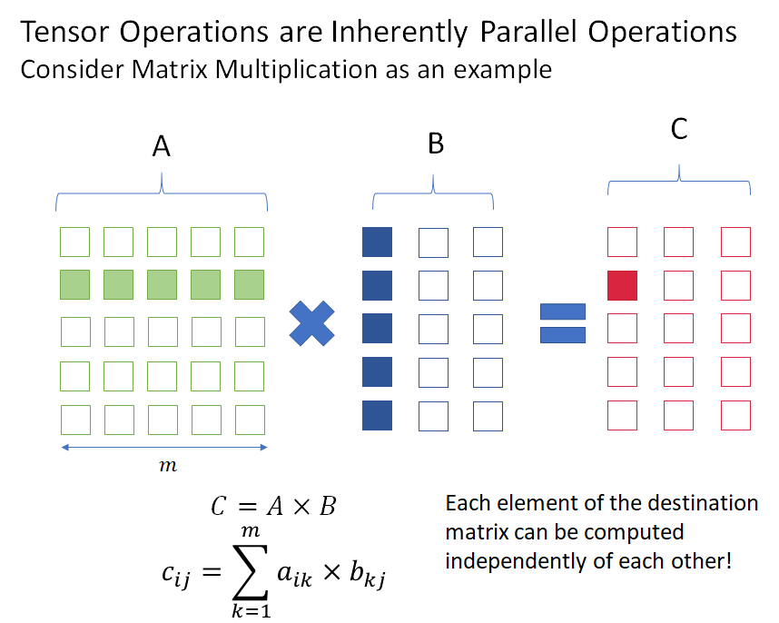
As a simple example, consider matrix multiplication (the fundamental operation in deep learning). Elements of the output matrix don’t depend on each other and can be computed in parallel, as shown in the figure below.
Because of this inherent parallelism, the key performance metric for GPUs is not just how fast an individual operation can be performed (measured by processor clock speed), but how many operations can be performed per unit time. This is where GPUs excel – they are able to perform many operations in parallel, even though the speed of an individual operation is usually lower than on a CPU. For example, the clock speed is 1.5 GHz for 1080Ti GPU, while it is 3.7 GHz for Intel® Core™ i7-4800MQ. Despite the lower clock speed, the 1080Ti GPU achieves 11340 GFLOPS while the CPU only does about 28 GFLOPS (see: https://setiathome.berkeley.edu/cpu_list.php)
FLOPS is not the end of the story – processors need data on which to perform calculations. It is no good having a fast processor if data can’t be fed to it fast enough. It will simply be spinning its wheels waiting for the data to arrive. The speed at which data is sent to the processor is measured by the memory bandwidth and is measured in bytes per second. Memory bandwidth depends upon where the data being accessed is stored. For example, if the data is stored in the cache, the bandwidth will be much higher than if the data has to be fetched from RAM. I will have to more to say about this a bit later.
FLOPS can thus be written as the following product:
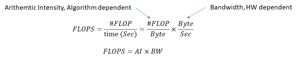
We introduced a new term here called “Arithmetic Intensity”. Arithmetic Intensity is algorithm specific and measures the number of operations per unit data. It is equivalent to “data reuse” i.e., the number of operations that can be performed before new data needs to be fetched. Some algorithms inherently have higher arithmetic intensity than others. As an example, let’s consider two operations:
- Matrix Addition: Let’s consider two
 matrices
  and
and  . For simplicity, we don’t care about the type of data in the matrices (byte, float etc). The matrix data first needs to be read from memory, undergo addition and then the resulting sum matrix written back to memory. The total amount of data transferred is therefore
  . Calculating the sum involves adding corresponding elements of each matrix and thus there are operations. The arithmetic intensity (AI) is therefore
  .
. - Matrix Multiplication: In this case, the amount of data read/written is the same as before. However, computing an element of the product involves
 multiplications and
  additions. Thus, the total amount of computation is
  (considering an addition and multiplication to be equivalent computations). The arithmetic intensity therefore is
  . Since the AI of matrix multiplication is proportional to the size of the matrix, large matrices have higher AI than small matrices. This is one of the reasons batching is so effective in deep learning – batched data is concatenated into large matrices which results in higher arithmetic intensities. Note that this analysis assumes that the matrix data is able to fit in available memory. This assumption is usually not true for large matrices. There is usually only a few dozen KB of high bandwidth shared memory available and matrices typically encountered in deep learning calculations can’t fit in shared memory. We’ll look at the implications of this in the last section.
Roofline Plots
Roofline charts were first introduced by David Patterson and others in 2008 in their ACM paper “Roofline: An Insightful Visual Performance Model
for Floating-Point Programs and Multicore Architectures”. Here’s the basic idea. We saw earlier that
 .
.
Taking log of both sides,

The plot of  against
  is called the roofline plot. Expressing the plot in the well known slope-intercept form
  , we immediately see that
  and
and  and thus the slope is 1 with intercept
  . Roofline charts start with a upward slanting line with slope 1 where increasing the AI leads to an increase in FLOPS until the peak FLOPS possible is reached after which the graph becomes flat. In this flat region, all available compute power is being utilized and increasing the arithmetic intensity doesn’t improve performance. The benefit of roofline plot is that they express the characteristic of the algorithm (Arithmetic Intensity) and the hardware (peak FLOPS and BW) in one graph, making it easy to see how to improve the performance of an algorithm and to compare the performance of different algorithms and hardware in the same plot.
To make these ideas more concrete, lets look at the contrived roofline plot below.
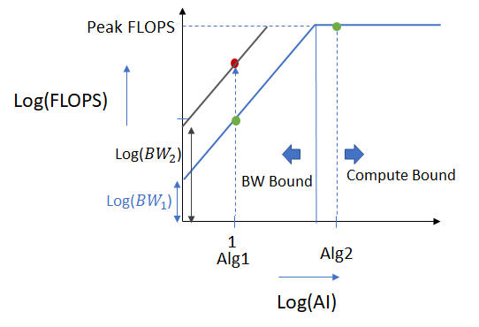
We consider two algorithms Alg1 and Alg2 with Alg2 having a higher arithmetic intensity. Alg 1 lies on the sloping part of the roofline chart and is called “bandwidth or memory bound”. This is because low memory bandwidth is preventing the algorithm from achieving the maximum possible performance this hardware offers. To improve the performance of the algorithm, we can either try to increase its AI (by using an implementation that achieves higher data reuse) moving it along the right along the x axis, or increase the memory bandwidth (by buying higher bandwidth memory or making more efficient use of cache) and moving it up. Increasing the memory bandwidth will improve the performance from the green to the red dot.
Alg2 has a higher arithmetic intensity and lies on the flat part of the roofline plot. By virtue of its higher AI, this algorithm uses more computation per unit data transferred and is already using all available compute resources and achieving peak FLOPS. To improve the performance of this algorithm, we’d need to invest in hardware with faster and/or larger number of computing resources.
We earlier noted that AI is a function of an algorithm while memory BW a function of the HW. This is not strictly true. There are multiple levels of memory hierarchies within a hardware and the effective memory bandwidth of an algorithm will depend on where the bulk of its data resides. Let’s consider the example of the data flow from a CPU to a GPU.
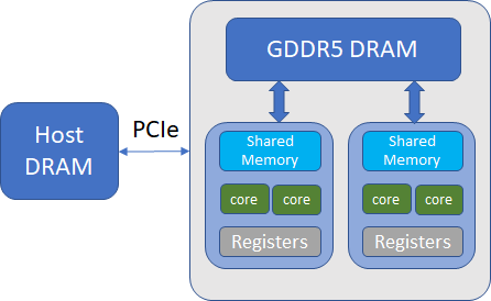
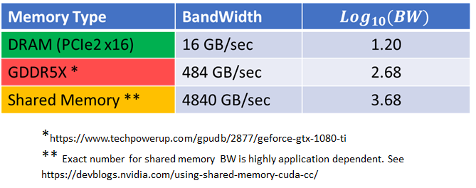
Broadly speaking, there are three memory types and associated data transfers involved. Initially, the data resides on the CPU main memory (for example when you training a CNN from images, you read the images from the disk and load the image data into main memory). This data is transferred over to the GPU global memory over the PCIe bus (this happens when you call .cuda() on the data tensor). When your program is running, the data in the GPU global memory is transferred to the shared memory located in the streaming microprocessors (this is done automatically by the underlying cuda implementation). As shown in the table below, the memory bandwidth gets roughly an order of magnitude larger as you get closer to the streaming microprocessor. This is accompanied by a corresponding decrease in the size of the memory available – Host DRAM is usually dozens of GB, Global GPU memory around 10 GB (on a 1080Ti GPU) and shared memory ~ 64 KB (per streaming microprocessor)
Let’s now look at the roofline chart for a 1080 Ti GPU with separate plots corresponding to each of memory types above. From the datasheet, the peak FP32 performance for this GPU is 11,340 GFLOPS. Plotting the data (roughly to scale) on the roofline chart, we get the following.
![]()
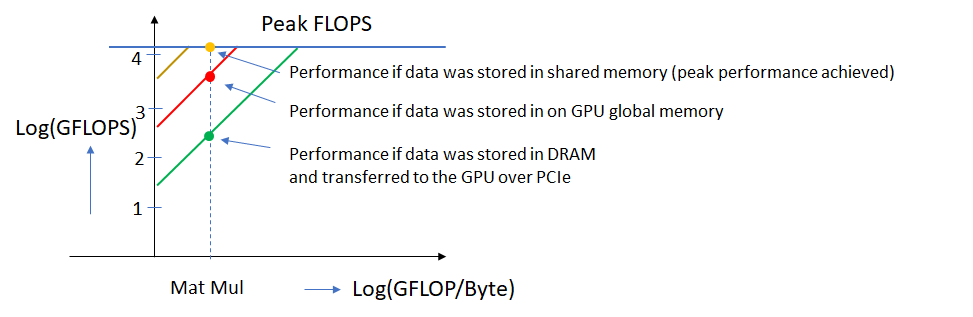
The green, red and yellow lines show the roofline plots for the three memory types. An algorithm would achieve different performance depending on where the bulk its data resides. In the example shown here, peak performance is achieved when the data is located in shared memory but not otherwise. This is one of the reasons why it is very important to use the right software libraries to achieve good performance from your hardware. Properly optimized libraries ensure that as much of the data as possible is read from the highest bandwidth memory available.
As another example, let’s look at the roofline plot in Google’s whitepaper about their “TPU” (Tensor Processing Unit).
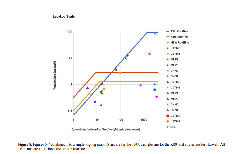
Part of the data used to construct this plot is given in table 2:
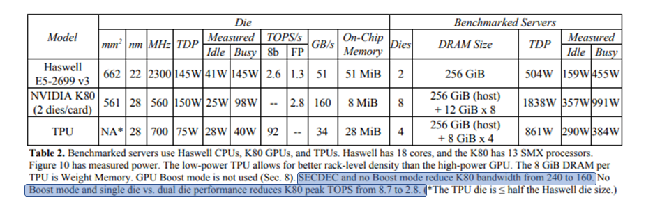
Notice how the hardware configuration can have a dramatic influence on achieved performance. Not using the “Boost mode” has a significant impact on peak FLOPS and BW for this GPU!
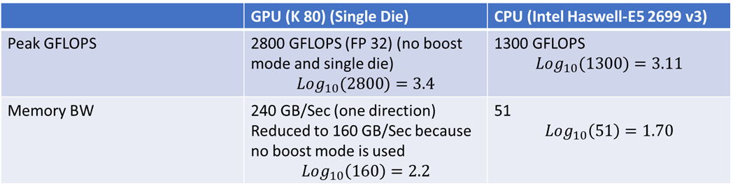
Isolating the data about GFLOPS and Memory Bandwidth, we get the following:
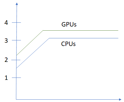
When we plot this data on the roofline chart, we get a shape that looks similar to the one shown in the paper.
Efficient Matrix Multiplication
While calculating the arithmetic intensity of matrix multiplication above, we assumed that the entire matrix data was available in the highest bandwidth memory. This is not the case for large matrices commonly encountered in deep learning calculations. For example, the size of shared memory available inside a streaming microprocessor on a GPU is usually around 100KB, while the size of a 3 channel  image is 270KB. If we implement matrix multiplication in a naive manner by repeatedly reading in rows and columns from slow global memory to fast shared memory, we lose the linear scaling with the matrix size as shown in the figure below.
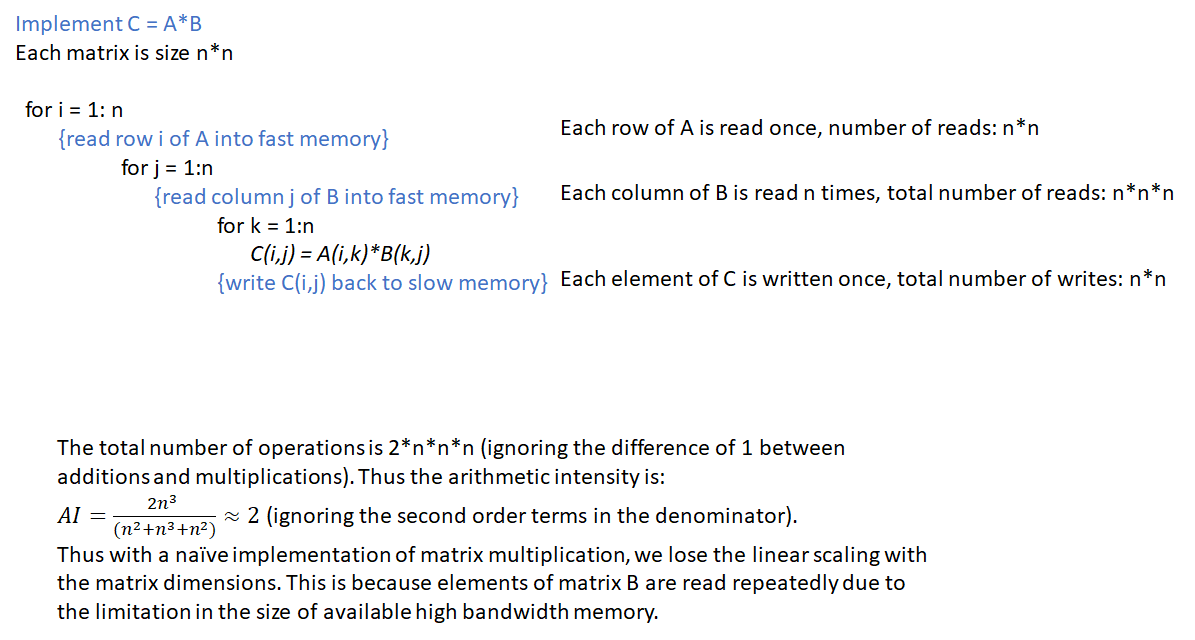
This problem can be addressed by using “Block matrix multiplication”, where blocks of rows and columns are read into memory and used to calculate partial sums of the output matrix. The details are described in many references on the web, see this for a nice explanation. The conclusion is that by using block matrix multiplication, the AI ~ b, the block size. The block size is chosen based upon the size of available shared memory, the number of threads in a thread block etc. A common size is 16. See this presentation for more details.
That’s it! Hopefully this information was helpful as a gentle introduction to roofline charts. I’ll add more info as my own understanding of roofline charts get better.
Your explanation is brilliant. I learned more by reading this than by reading 3 different papers. You save my day! Thank you
Thanks! Glad you liked the post.
This is amazing stuff. Thanks for taking the time and making it look so easy.
Just wondering which tools did you use to generate graphs and equations?
Glad you liked the post. I used Latex for WordPress for the equations. It supports pretty much all of Latex
Really awesome and well explained article. Thanks so much, there are lots of small details I didn’t understand but they are explained very clearly here!