

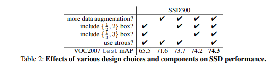
Over the past few days, I have been investigating how SSD (Single Shot Detector), an object detector introduced in the following paper (https://arxiv.org/pdf/1512.02325.pdf) in Dec 2016 that claims to achieve a better mAP than Faster R-CNN at a significantly reduced complexity and achieves much faster run time performance. I’ll describe the details of SSD in a subsequent blog. The purpose of this blog is to describe the data augmentation scheme used by SSD in detail. According to the paper, the use of data augmentation leads to a 8.8% improvement in the mAP.
Data augmentation is particularly important to improve detection accuracy for small objects as it creates zoomed in images where more of the object structure is visible to the classifier. Augmentation is also useful for handling images containing occluded objects by including cropped images in the training data where only part of the object may be visible.
Table of Contents
Data Augmentation Steps
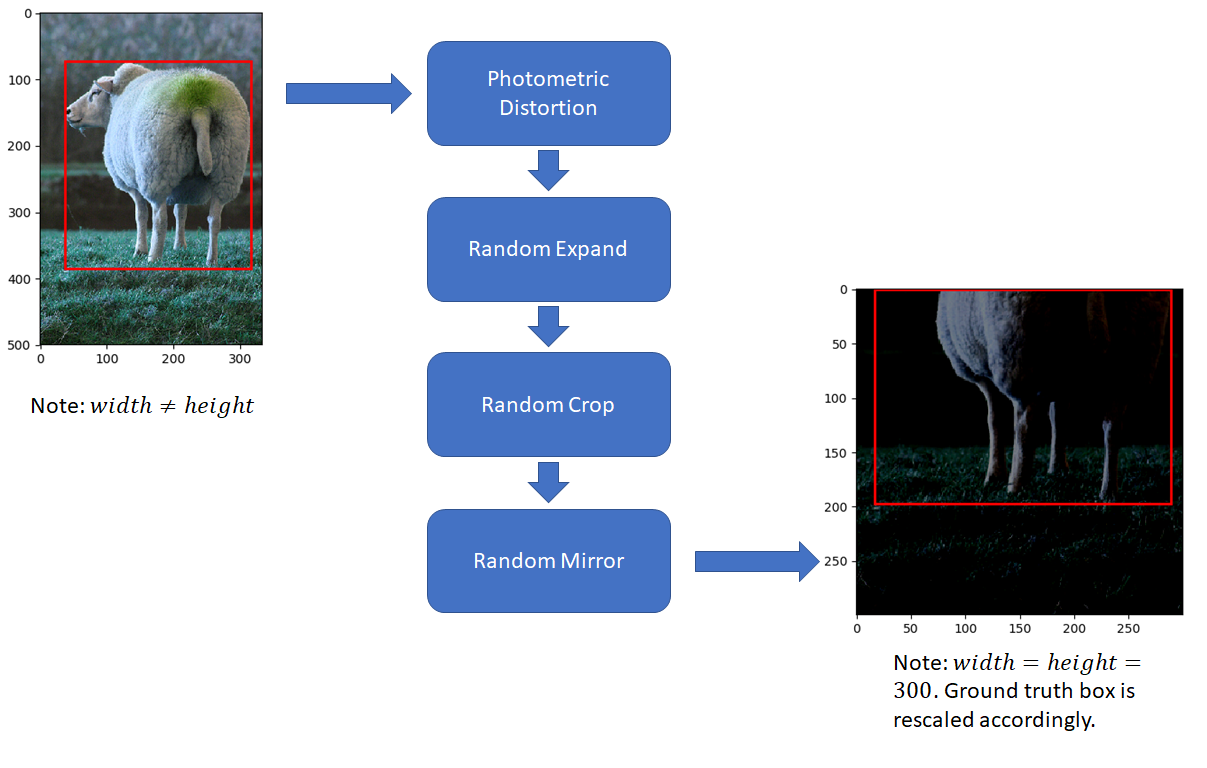
The following data augmentation steps are used and are applied in the order listed.
- Photometric Distortions
- Geometric Distortions
- ExpandImage
- RandomCrop
- RandomMirror
In the sections below, I’ll describe these steps in more detail. Note that each distortion is applied probabilistically (usually with probability = 0.5). This means that different training runs will use different image data that results from the augmentation steps applied to the original training data. I will also include the relevant code snippets, making it easier to connect the algorithm with the code that implements it. I’ve used the following PyTorch code repository in my experiments – https://github.com/amdegroot/ssd.pytorch/
Photometric Distortions
Random Brightness
With probability 0.5 (see documentation for random.randint for why “2” is passed as an argument), this function adds a number selected randomly from [-delta, delta] to each image pixel. The default value of delta is 32
|
1 2 3 4 5 |
def __call__(self, image, boxes=None, labels=None): if random.randint(2): delta = random.uniform(-self.delta, self.delta) image += delta return image, boxes, labels |
Random Contrast, Hue, Saturation
After applying brightness, random contrast, hue and saturation are applied. The order in which these are applied is chosen at random. There are two choices – apply contrast first and then apply hue and saturation or apply hue and saturation first and then contrast. Each choice is made with probability 0.5, as shown in the code below
|
1 2 3 4 5 6 7 8 9 10 11 12 13 14 15 |
self.pd = [ RandomContrast(), ConvertColor(transform='HSV'), RandomSaturation(), RandomHue(), ConvertColor(current='HSV', transform='BGR'), RandomContrast() ] im, boxes, labels = self.rand_brightness(im, boxes, labels) if random.randint(2): distort = Compose(self.pd[:-1]) else: distort = Compose(self.pd[1:]) im, boxes, labels = distort(im, boxes, labels) |
Note that contrast is applied in RGB space while hue and saturation is applied in HSV space. Thus the appropriate color space transformation must be performed before each operation is applied.
Application of contrast, hue and saturation is done in a manner similar to brightness. Each distortion is applied with probability 0.5, by selecting the distortion offset randomly between an upper and lower bound. The code for applying saturation distortion is shown below.
|
1 2 3 4 5 |
def __call__(self, image, boxes=None, labels=None): if random.randint(2): image[:, :, 1] *= random.uniform(self.lower, self.upper) return image, boxes, labels |
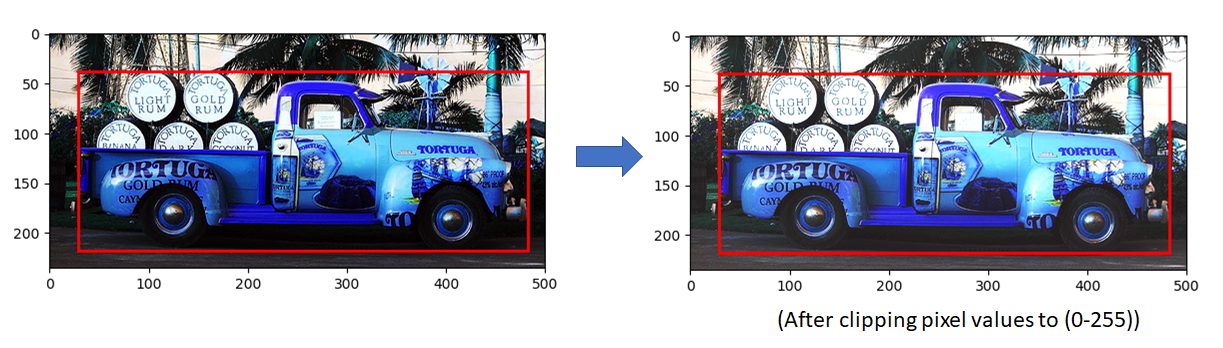
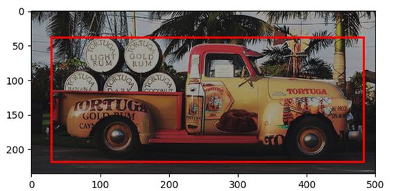
The image below shows the result of applying some of these distortions (I’m not sure which ones were applied since the choice is made randomly)
RandomLightingNoise
The last photometric distortion is “RandomLightingNoise”. This distortion involves a color channel swap and is also applied with probability 0.5. The following color swaps are defined:
|
1 2 3 |
self.perms = ((0, 1, 2), (0, 2, 1), (1, 0, 2), (1, 2, 0), (2, 0, 1), (2, 1, 0)) |
For a RGB image, the swap (0 2 1) would involve swapping the green and blue channels, keeping the red channel unchanged. The swap that is actually applied is chosen randomly from this array.
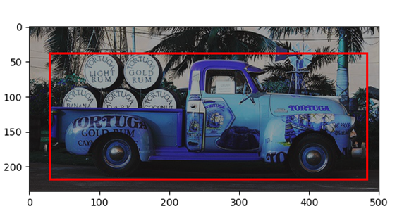
The image produced after applying one of these swaps is shown below:
Geometric Distortions
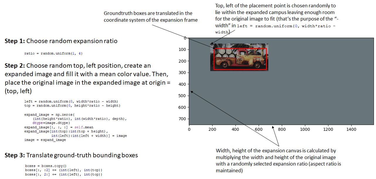
RandomExpand
Unlike photometric distortion that changes the image pixels but not the image dimensions, the next few augmentation steps are geometric and involve change in the image dimensions. We’ll first consider RandomExpand followed by RandomCrop and RandomMirror. The steps carried out in RandomExpand are shown in the figure below. As with photometric distortion, RandomExpand is applied with probability 0.5
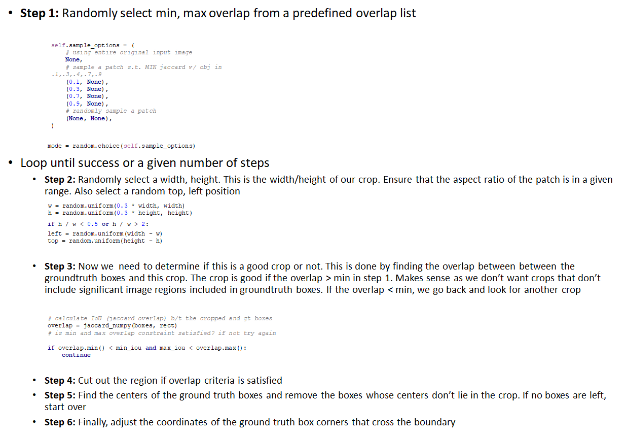
RandomCrop
The goal of this step is to crop a patch out of the expanded image produced in ExpandImage such that this patch has some overlap with at least one groundtruth box and the centroid of at least one groundtruth box lies within the patch. This requirement makes sense as patches that don’t contain significant portion of foreground objects aren’t useful for training. At the same time, we do want to train on images where only parts of the foreground object are visible. The steps carried out in RandomCrop are shown in the figure below.
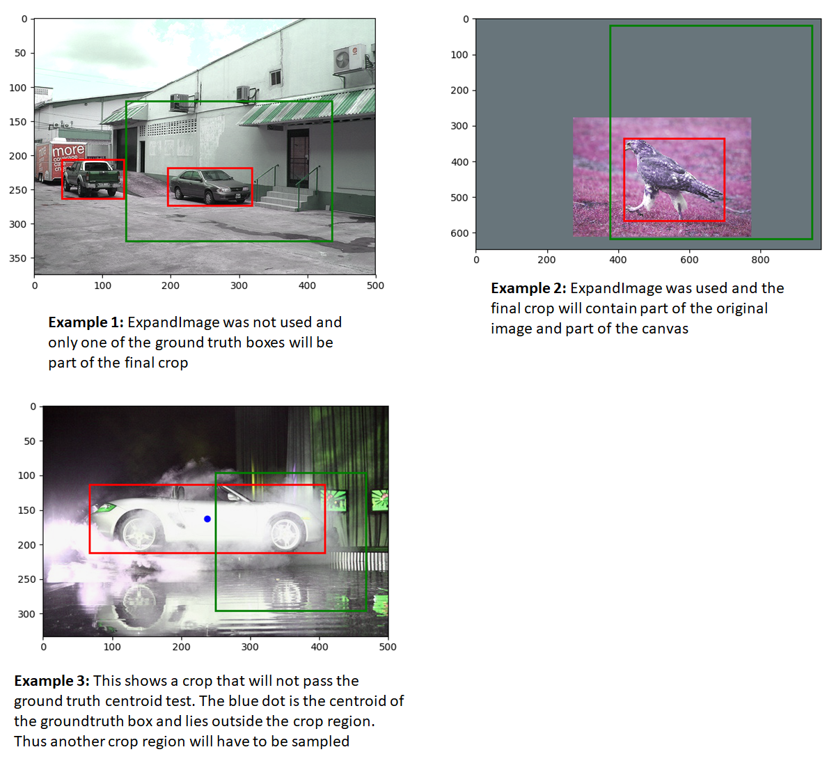
Let’s now look at a few examples to further illustrate these ideas. Ground truth boxes are shown in red while the cropped patch is shown in green in the images below. Recall that the RandomCrop step follows the ExpandImage step, which is applied with probability 0.5. So some of these images have an expansion canvas around them, while others don’t.
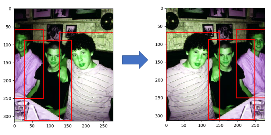
RandomMirror
The last augmentation step is RandomMirror. This one simply involves a left-right flip and is a common augmentation step used in other object detection and image classification systems also.
Finally, as in other object detection and image classification systems, the image is resized to 300, 300, ground truth coordinates are adjusted accordingly and normalized and mean is subtracted from the image.
Hi
Did not understand RandomExpand
Is the process creating a blank image and placing a small version of original image on it?
That’s correct, except the original image is placed in the expanded campus, not a smaller version of it (at least in the implementation that this post refers to)