

Recently, I’ve been learning about sequence-to-sequence translation systems and going through Pytorch’s fairseq code. I’ve been focusing on the convolutional seq-to-seq method by Gehring et al. The basic idea behind seq-to-seq models is easy to understand, but there are a number of issues in the implementation that I found tricky to understand. In this post, I’ll elaborate on some of these issues.
- Use of padding in the linear convolution layer used in the encoder
- Operation of the GLU layer
- Use of padding in the decoder during training
- Preventing the right to left flow of information during training
- Incremental decoding used to speed up inference
- how does incremental decoding speed up inference?
- why is reordering of incremental state needed?
- why does the beam search return results that are twice the number of beams and a few other smaller points.
I won’t describe how convolution based seq-to-seq training and inference and associated algorithms such as beam search themselves work. The original paper does a great job at describing how the method works and several blog posts and presentations on the web provide additional details. I’ll focus on issues I found tricky to understand as I was stepping through the Python code, particularly how padding is used and how the incremental decoder works. I found the code author’s answers to some of the fairseq github issues quite helpful. Those answers should be included in the fairseq documentation :). Stepping through the Python code, inspecting the size of tensors and understanding how information flows through the network is a great way to develop a full understanding of how ML algorithms work. I recommend doing so as you are going through the material in this post.
I thank Facebook’s AI team for making fairseq available. Making high quality, almost production ready implementations of state of the art sequence-to-sequence methods available is a great service to the ML community. The tech companies get a lot of bad press related to their handling of user data, but their important contributions to the research community through high quality ML libraries such as Pytorch and Tensorflow and implementations of important ML algorithms doesn’t get much attention. So, thanks again Facebook AI team for Pytorch and fairseq 🙂
I’ll start by providing a brief overview of the major milestones in neural network based machine translation. This overview provides a high-level view of the progress in this field by describing the key improvement made in each milestone and is not meant to be exhaustive.
Table of Contents
Progression of Neural Machine Translation
LSTM/RNN based Encoder-Decoder systems
Neural Machine Translation (NMT) has achieved dramatic success in language translation by building a single large network that reads a sentence and outputs a translation and can be trained end-to-end without the need to fine tune each component. The first successful NMT systems used an encoder-decoder architecture where the encoder neural network (typically a LSTM or RNN) reads and encodes a source sentence into a fixed-length vector. A decoder then outputs a translation from the encoded vector. The whole encoder–decoder system is jointly trained to maximize the probability of a correct translation given a source sentence.
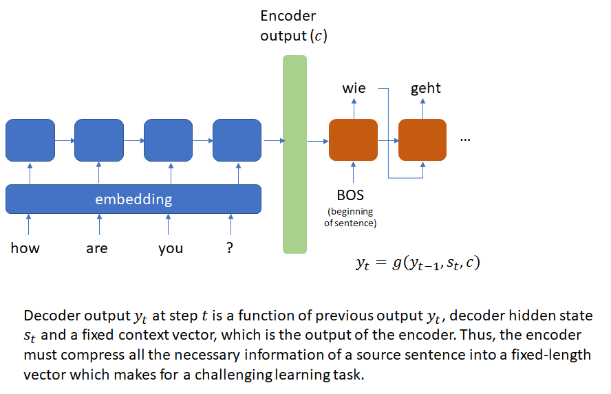
This system presents a difficult learning task as the encoder must compress all the necessary information about a source sentence into a fixed length vector.
Attention mechanism
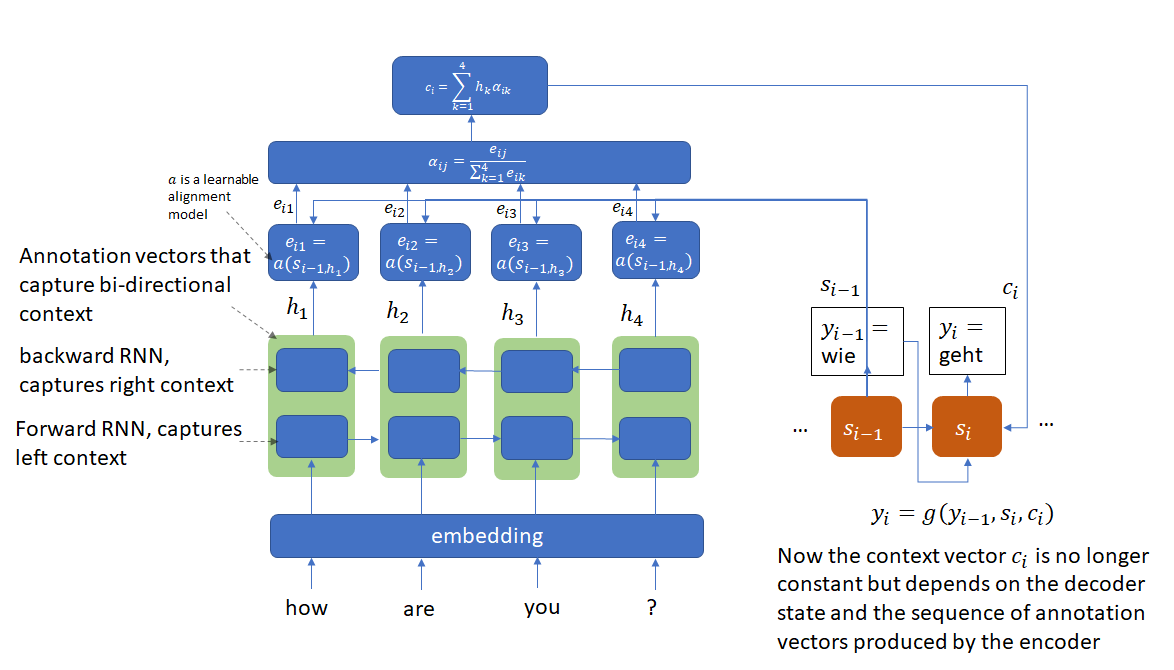
To address this issue, Bahdanau et. al. introduced the attention mechanism that encodes the input sentence into a sequence of vectors and uses a linear combination of these vectors while decoding the translation. The coefficients of this linear combination are called attention scores and depend on the decoder state. The attention mechanism allows the network to focus on different parts of the input sequence as it generates the output sequence. This approach obtained BLEU scores almost 10 points higher than the previous approach (that didn’t use attention) and matched the performance of traditional phrase-based approaches.
Removing recurrence: Transformer and convolutional architectures
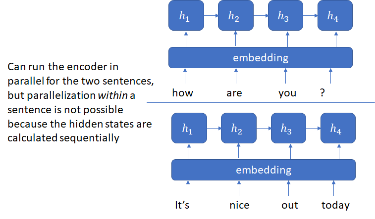
The next major advancement was the transformer architecture that avoided the recurrence inherent in RNN and LSTM based architectures and instead relied entirely on an attention mechanism to draw global dependencies between input and output. The problem with recurrence is that the hidden state  depends on the input at position
  and previous state
  which inherently precludes parallelization within training examples.
The transformer model surpassed the previous state of the art based on recurrent architectures in performance and significantly lowered the training time by making it possible to parallelize both across and within input sentences. Transformer model and its successors continue to be popular GMT models. The original transformer model is included in the reference NMT models used by MLPerf for ML HW performance evaluation.
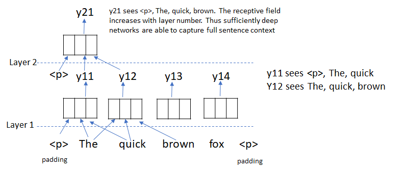
Another method to capture context while avoiding recurrence is using 1D convolutions. This approach was pioneered by Dauphin et al. in Convolutional Sequence to Sequence Learning. Just like with 2D convolution on images, the receptive field (i.e., the number of words a convolution kernel “sees”) of a convolution kernel increases with depth and thus by stacking multiple convolutional layers, the full sentence context can be captured without the need to use recurrence.
The authors also introduce a simple gating mechanism called Gated Linear Units (GLU). These units retain the non-linear capabilities of the layer while allowing the gradient to propagate through without scaling and eliminate the need for the input and forget gates used in LSTMs to solve the vanishing gradient problem. See original paper for details on how this works.
Convolutional seq-to-seq encoder
I’ll now describe a couple of issues with the implementation of convolutional seq-to-seq encoder that took me some time to understand as I was going through the code. The first issue is how padding is used and the second is the operation of the linear convolution and the GLU layer. If you are not familiar with the convolutional encoder-decoder, read the original paper first and run the training code following the directions here to become familiar with the model architecture.
Use of padding in the encoder
Consider the use of padding in the encoder and decoder in the seq-to-seq model. The model architecture shown below is taken from the original paper.
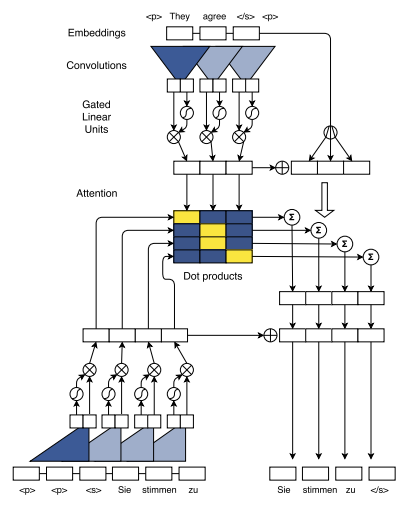
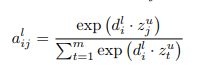
Notice that the source sentence uses padding of size = 1, while the target sentence uses padding of size 2. Let’s consider the encoder first. The use of padding is easy to understand if one focuses on the output of the encoder. The goal of the encoder is to produce the key, value vectors for each source word that are used to produce attention scores and conditional input for each decoder layer. The relevant equations are shown below (refer to the original paper):
Here  denotes the current decoder layer,
  is the decoder summary vector for state
  and layer , and
  is the encoder output for source word and encoder block
  , which is always the last encoder block in this implementation. The summation is over
  , the number of source words. Thus, for the dimensions to work, the size of the encoder output must be
  ( vectors of dimension
  ).
).
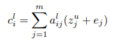
The second use of the encoder output is to compute the conditional input  for the decoder which uses the attention scores calculated above as the weights and vectors
  as the values. Here
  is the encoder output for source word
  and encoder block (as above) and
  is the source word embedding.
Thus, the encoder should produce two matrices of  and
and  vectors, of equal dimensions.
Let’s now consider how the source data is processed by the encoder. The first step is to convert the source words into their indices in the word vocabulary followed by embedding lookup. The embedding vector values shown below are arbitrary numbers. The dimension of the embedding vector is the default value in the fairseq implementation.
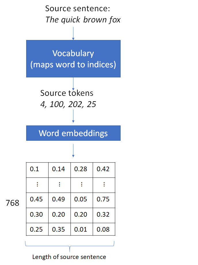
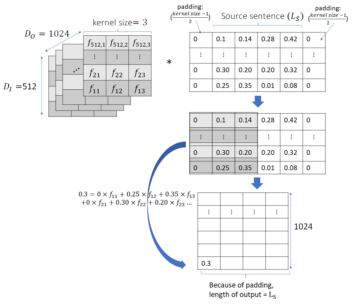
This results in a matrix where the columns are the embedding vectors for each source word. This is followed by addition of the positional embedding and dropout, which are point-wise operations and don’t change the matrix dimensions. The next operation is the 1D convolution that can change the matrix dimensions, depending on the number of input and output features and the filter kernel size. A 1D convolutional filter bank of output feature size  consisting of
  kernels operating on
  input produces output of size
  . Here
  are the kernel width, padding and stride respectively. We want the number of output words to be same as the input and thus
  for
for  . So this explains why padding of size 1 is used in the source sentence. We want the length of the input to stay the same as it moves through the network. The figure below shows the operation of 1D convolution.
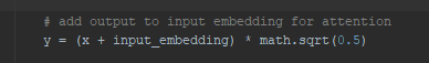
GLU layer
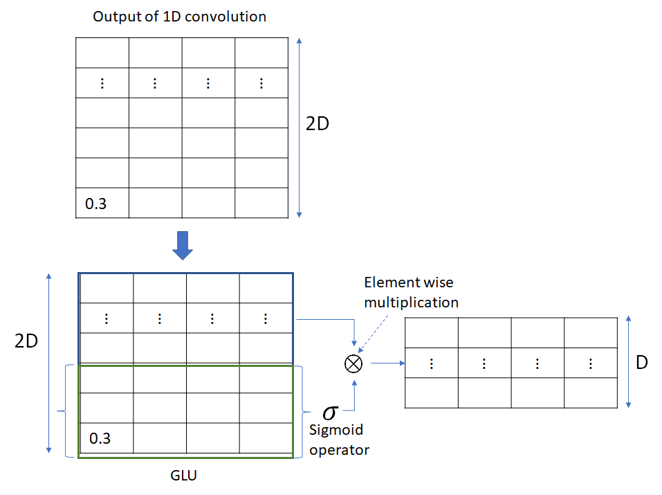
1D convolution is followed by the GLU layer which applies a gating operation on each column that halves the dimension of the column, as shown below. Unlike the preceding 1D convolution layer, GLU doesn’t mix information across columns.
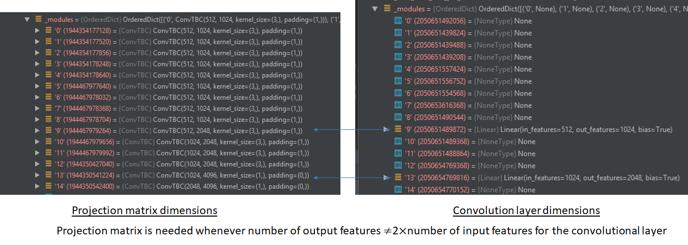
Accounting for the halving of output dimension caused by the GLU layer, the output of the convolutional layer is chosen to be twice the desired output at the end of the GLU layer. To facilitate training of deep convolutional networks, residual connections are added from the input of each convolution to the layer’s output. The combination of dropout, 1D conv and GLU constitutes a block. The default fairseq implementation uses 15 such blocks chained together. Convolutions in some of the later blocks cause a change in the output dimensions. In those cases, projection matrices are used in the residual connections to perform the required dimension projection. The complete encoder architecture is shown below. The numbers shown are the default values used in the Pytorch fairseq implementation. The architecture shows the data flow for a single source sentence (batch size = 1).
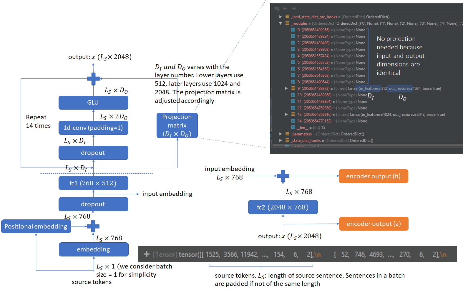
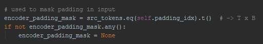
The implementation works on batches of source and target sentences and not all sentences are of the same length. The shorter sentences are padded so that all sentences in a batch are the same length. A padding_mask is created to note the places where padding is used.
Finally, you’ll see multiplication with scaling factors wherever multiple inputs are combined. This is to prevent a change in variance between the input and output.
This also applies to initializing weights for various layers. The weights should be initialized such that the the variance of activations throughout the forward and backward passes is maintained. The original paper provides detailed proofs for the scaling factors in the appendix.
Convolutional seq-to-seq decoder
I found two issues with the decoder architecture during training tricky to understand. The first is the right shifting by one position of the target word sequence and the second is use of padding to prevent right to left flow of information.
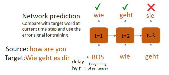
Right-shifting the target sequence
The first issue is easier to understand using the example of a RNN decoder. Remember that during training, the decoder’s is asked to predict the word at the current time step. The difference in the decoder’s output and the correct word provides the training signal. In making its prediction, the decoder must only use words in the target sentence prior to the current word, because clearly if the decoder is shown the current word in the target sequence, the decoder will soon learn to just use that and ignore all other information presented to it. To keep the decoder from seeing the current word, the target word sequence is time shifted by one unit.
Use of padding in the decoder
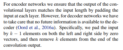
In a convolution-based architecture where the target sequence is processed at once instead of sequentially, an additional issue arises. We must also prevent information flow from right to left to avoid exposing information about future words to parts of the network tasked with predicting those words. In the transformer model, this is achieved through masking. In convolution based networks, this is done through a clever use of padding. Recall that in the encoder, we used padding = 1 for convolutional kernel size = 3. This was done to preserve the size of the convolution output to be same as the input. In the decoder, we use padding = 2 on the left and right and discard the last two elements of the convolution output. This construction applies a leftward pressure on the receptive field so that convolution filters are prevented from seeing information about words they’ll be asked to predict. The figure below how this works for 2 convolution layers. The figure shows the convolution operation only and ignores the others layers (GLU, attention) which don’t involve mixing of information across target sentence words.
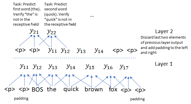
The original paper expresses this idea as shown below. I hope my explanation makes this a bit easier to understand 🙂
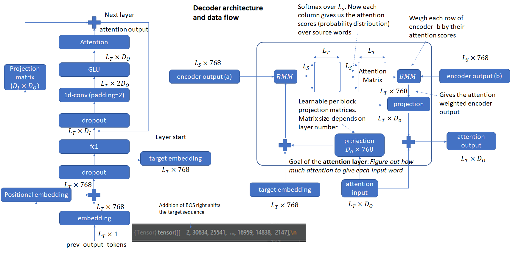
The complete decoder architecture is shown below. Note the use of encoder outputs that we saw earlier. The architecture is very similar to the encoder. The differences are the use of right shifted target input, use of padding = 2 and computation of per-layer attention scores.
Incremental Decoding during Inference
During inference (language translation in the case we consider here), the decoder outputs the probability distribution over the target language vocabulary at each time step. The simplest translation algorithm simply selects the most likely target word in a greedy manner. This approach mirrors the loss function used during training. At the other extreme, one could collect all possible target sequences and pick one that minimizes the overall log likelihood. Doing so involves searching through all the possible output sequences based on their likelihood. Since the size of the vocabulary is often tens or hundreds of thousands of words, the search problem is exponential in the length of the output sequence.
Beam search is a compromise between these two extremes. I won’t go into the details of how beam search works, as there are a number of excellent tutorials on the web. Beam search is significantly more efficient than an exhaustive search because we must only consider  prefix sequences at each time step and the search space is
  instead of
  where is the beam width and
  is the target vocabulary. One drawback of beam search is the lack of diversity in decoded solutions. This is suboptimal for language translation where a given source sentence can have multiple correct translations. Several solutions have been proposed to enhance the diversity of solutions found by beam search. Diverse beam search adds a dissimilarity term to the standard beam scores that encourages more diverse beams by penalizing words used in previous steps and top-k random sampling where the tokens for the next generation are randomly sampled from the top-k most likely candidates (instead of always picking the top candidates).
While beam search is more efficient than brute force search, the search overhead still increases linearly with the length of the decoded sentence, because at each time step, we must consider all prefix tokens.
In this example, I’m using letters A, B, C etc. to denote word tokens. A cool trick used during inference is that beams are expanded into the batch of sentences being translated. So if my input batch consists of two sentences and the beam size is 3, the batch will be expanded to size 6, so that each beam is processed in parallel as a batch element.
Since we have already run the decoder for the previous tokens, couldn’t we simply reuse that calculation? That’s exactly what incremental decoding does. An incremental_state data structure maintains a history of previous calculations that are needed for calculating the convolution output. The decoder is only run on the tokens in the current time step and layers such as convolution that need previous token state can get it from the incremental_state. Since the encoder doesn’t depend on the target sequence that is being decoded, it is run on the source sentence at the beginning to generate the (key, value) encodings for each source word which are then reused by the decoder.
How does incremental decoding save computation?
The actual implementation of incremental decoding is a bit tricky, hopefully the figures below will make it easier to understand. I recommend running the code in the python debugger and setting breakpoints at the places shown below. That will make it easier to understand what happens at each step.
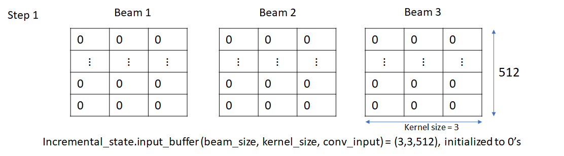
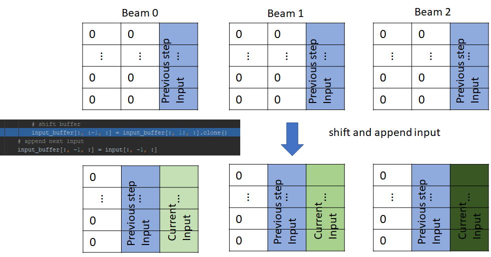
We’ll consider a single source sentence, so our batch size is equal to the beam size (3 in this example). Initially, each beam consists of the beginning of sentence (BOS) token. Thus embedding vectors at the input of the convolution layer are identical.
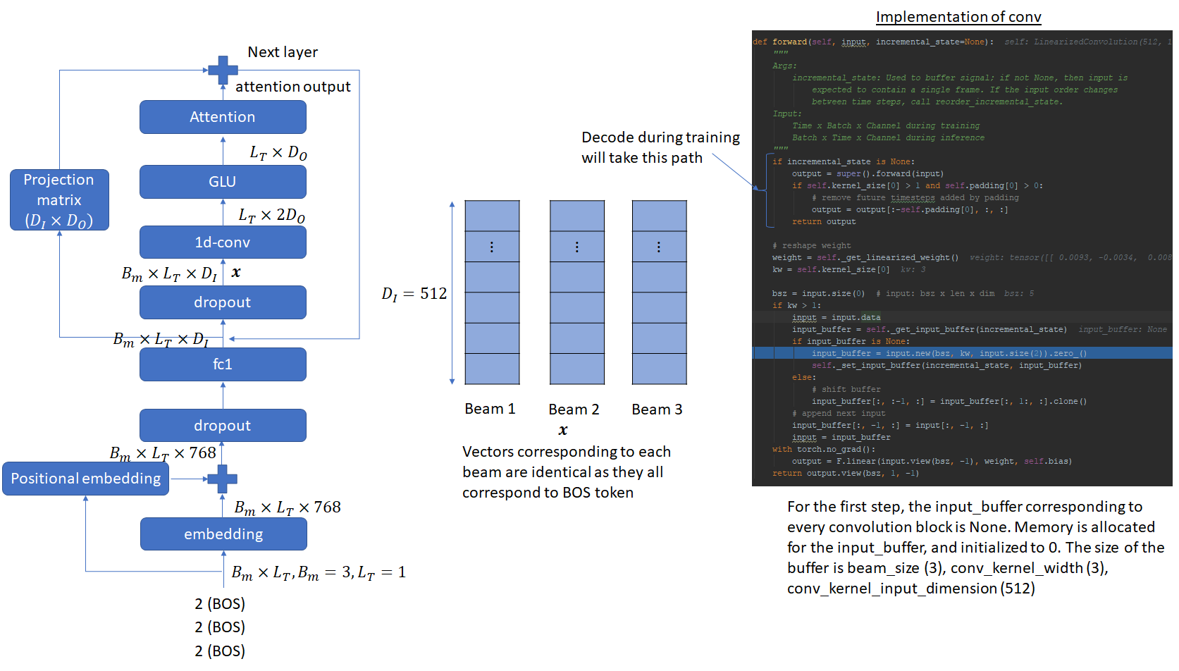
Here’s how the input_buffer looks like after creation and initialization
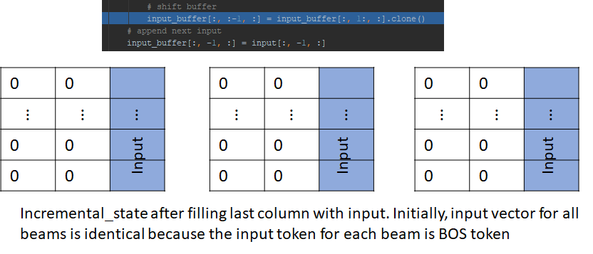
Next, the input_buffer is left shifted by one position and the input is appended to the last column. The left shifting doesn’t do anything in this step as the buffer is filled with zeros, but we’ll see its effect in the next step.
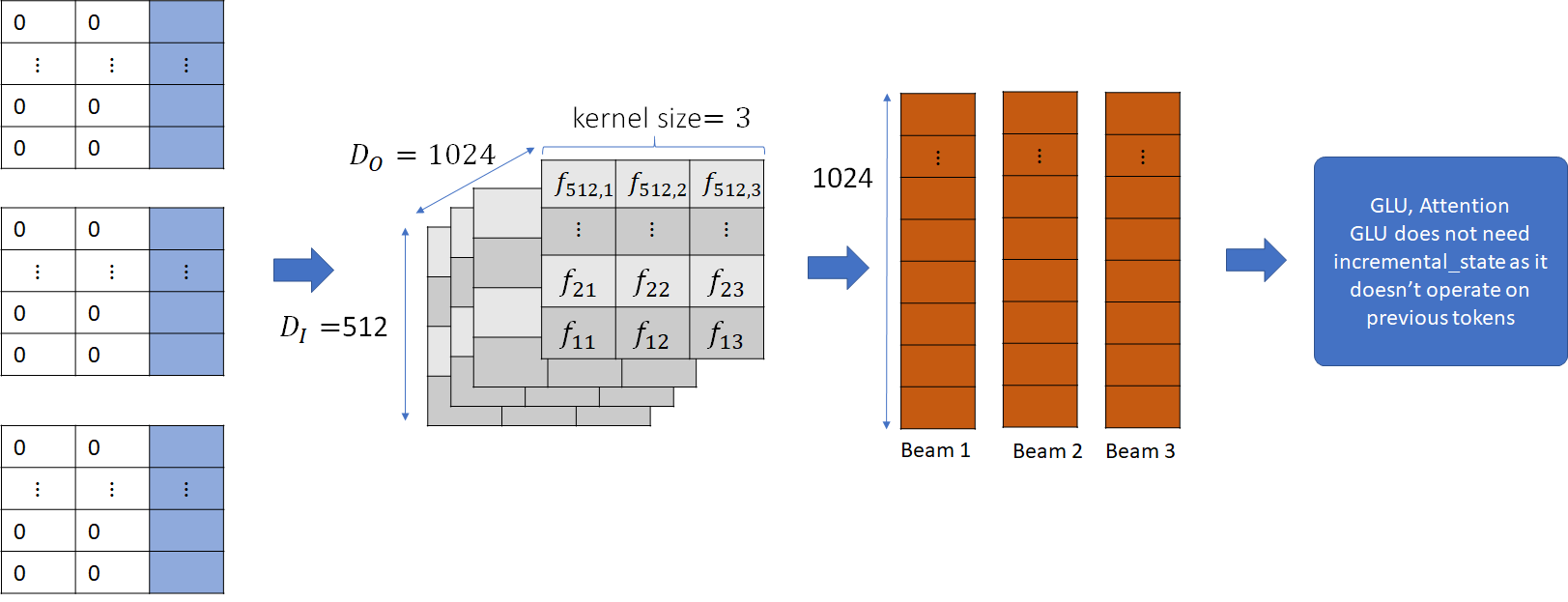
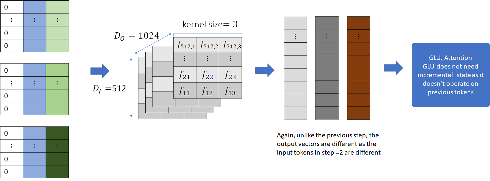
Next, the input is convolved with the convolutional filter and the output is passed to the subsequent layers – i.e., GLU and attention mechanism.
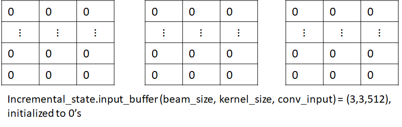
Let’s now consider the linear convolution layer in the next block. The input to this layer is the output of the previous block. Just like the convolution layer in the previous block, it has its own incremental state which is initialized to 0 and then filled with the input.
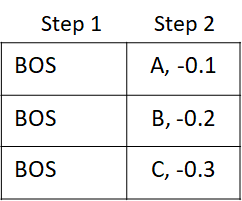
The input is then convolved with the convolutional kernel for this layer and passed to the GLU and attention layer, just like before. This process is repeated for all the blocks in the decoder. The output is the probability distribution vector over the vocabulary for each beam. This is passed to the beam search algorithm, which returns the best performing tokens for the next step. Let these tokens be A, B and C.
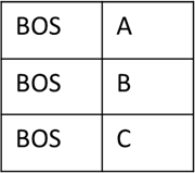
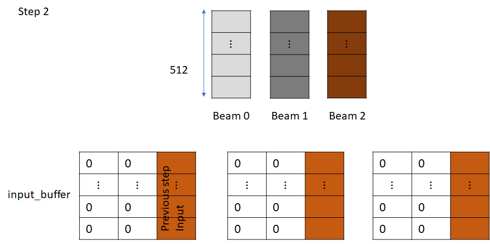
Let’s now consider what happens in the next step (2). Our beam looks like this:
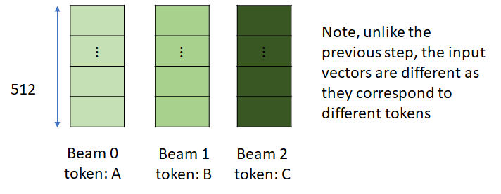
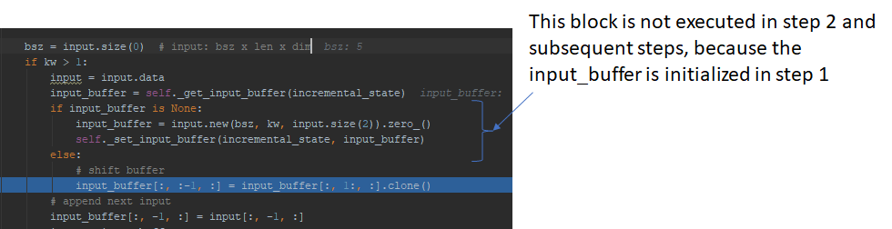
Let’s again consider the input to the first convolutional layer. Now, since the input tokens are different for each beam, the embedding vectors in the input are no longer identical. Also, the input_buffer for the incremental_state is no longer None as it was initialized in the previous step.
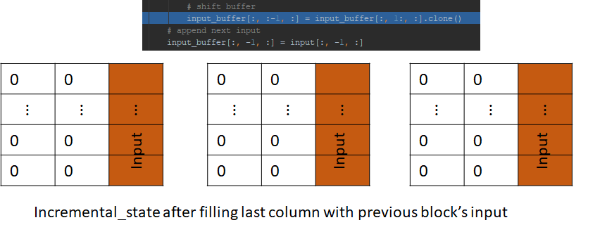
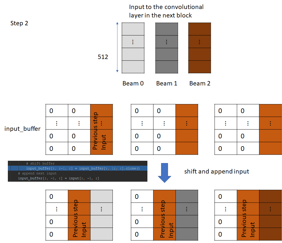
Next, the input_buffer is left shifted, and the new input is appended to the last column
The input_buffers for each beam are now convolved with the convolutional kernel and the output is passed to the subsequent layers, just like before.
This shows us how the input_buffer acts as a memory to remember the previous step’s input which is needed to compute the output of the convolution. The input_buffer also saves us computation, this becomes clear when we look at the operation of the convolution in the next block.
The incremental_step.input_buffer already contains the input from the previous step, which is needed to perform the convolution at this step. Crucially, this input is the output of the previous block and saving this input avoids needing to recalculate it, which would have required running the decoding process for the previous token. This is how incremental decoding saves computation. Rest of the process is same as before. We left shift and append input, execute the convolution and so on.
Reordering of incremental state: Why is it needed?
At the beginning of each step, the generator reorders the decoder’s and encoder’s incremental_state.
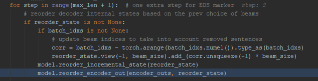
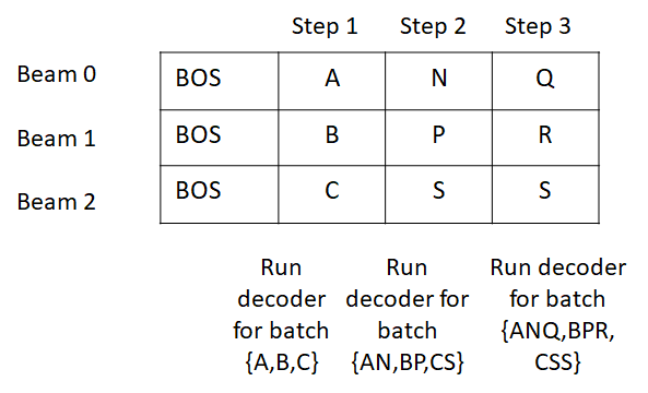
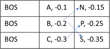
This is needed because beam search can result in a change in the order of the prefix tokens for a beam. Its easiest to see this through a simple example. Lets consider the beam state after step 2. The state shows the tokens and score for each step.
Now at step 3, tokens N, P, S are selected with the following scores. The arrows show the beam index each output token came from.
This results in the reordering of the beams as follows.
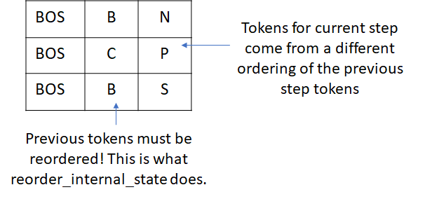
Now when we run the decode step for the current set of tokens (N, P, S), we must reorder the incremental_state so that the convolutions use the reordered prefix tokens. This can take some time to sink in so ponder it for a bit if it doesn’t sense immediately 🙂
Note that the fairseq code also reorders the encoder state, however since the encoder state only depends on the source tokens and not on the beam state, the reordering is not required, at least for the algorithm that I’m considering here.
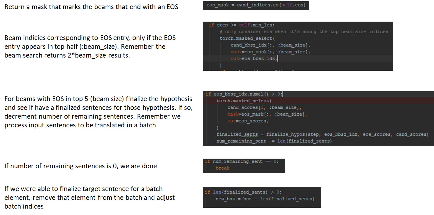
Why does beam search return twice the number of tokens as the number of beams?
Notice that in the fairseq implementation, beam search returns output tokens that are twice the number of beams. This is because the beam search could return end of sentence (EOS) token for some beams and we don’t want to terminate the beam search too early. When an EOS appears in the top half of the beam search results, we consider the corresponding hypothesis for sentence completion by comparing the total score for the hypothesis with other scores seen so far. I’ll show some relevant code below with helpful comments that make it a bit easier to follow.
That’s it! I hope this post will help clarify some of the implementation details in fairseq.
Thanks a lot for this awesome explanation. It saved my day. You should consider contributing this to the fairseq documentation.
Thanks and glad you found the post useful. Fairseq docs already refer to this post in the section about incremental decoding, here’s the link:
https://fairseq.readthedocs.io/en/latest/models.html#incremental-decoding
This is awesome explanation..
Thanks, glad you found it useful.
Thanks for the post. A small mistake here:
Beam search is significantly more efficient than an exhaustive search because we must only consider B prefix sequences at each time step and the search space is B\times V instead of V \times V where B is the beam width and V is the target vocabulary.
We are considering O(V^k+1) prefixes in exhaustive search when trying to decode the k+1th word.