

In this post, I’ll describe how to use distributed data parallel techniques on multiple AWS GPU servers to speed up Machine Learning (ML) training. Along the way, I’ll explain the difference between data-parallel and distributed-data-parallel training, as implemented in Pytorch 1.01 and using NVIDIA’s Visual Profiler (nvvp) to visualize the compute and data transfer operations involved.
Let’s motivate the problem first. Consider the time to train Resnet-50 on the Imagenet dataset, consisting of about 1.3 Million images. From my testing, time to run backprop on a batch of 64  images is on a 1080 Ti GPU is 0.328 seconds. Thus the time to run one epoch is
  = 1.85 hrs. It typically takes ~100 epochs for training to converge. Thus the total time to train is 185 hrs or around 7.7 days. Such a long training time is clearly unacceptable.
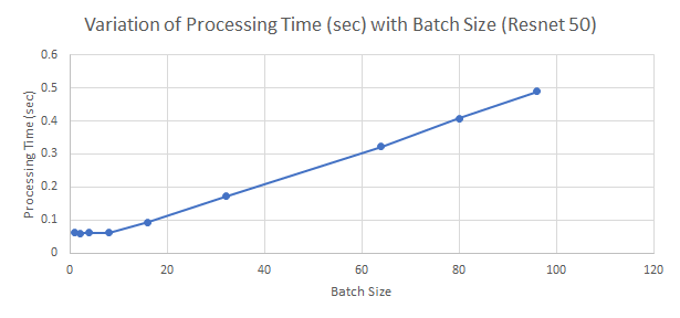
The sheer volume of compute required for training DNNs on large input batches is so large that the available parallel compute on even massively parallel computers such as GPUs is quickly exhausted. The plot below shows the processing time (forward +backward pass) for Resnet 50 on a 1080 Ti GPU plotted against batch size. Up to about a batch size of 8, the processing time stays constant and increases linearly thereafter. This is because the available parallelism on the GPU is fully utilized at batch size ~8.
Data parallel techniques make it possible to use multiple GPUs to process larger batches of input data. The basic idea is that if my training data set has  images, I split these up in batches of size
  and the time to process a batch is
  , then I can process one epoch in time
  . Now if I split up my data set into larger batches, say of size
  and I can process these larger batches in time
  , then my epoch time will be
  , lower almost by a quarter. The key is to keep the batching overhead
  as small as possible.
Recall that Minibatch Stochastic Gradient Descent (MB-SGD, or simply SGD) the algorithm used during DNN training averages the gradient across a batch before computing the parameter updates. When we increase the batch size, the average is performed over a larger number of elements. In the limiting case, if the batch size = size of training dataset, SGD becomes simple gradient descent as each batch consists of the same elements. As batch size gets larger, we must ensure that training accuracy and generalization performance is maintained. This great paper from Facebook AI shows how to scale the learning rate and other hyper-parameters to maintain accuracy and generalization performance. The paper shows that batch size for Resnet style networks can be scaled to about 8K before performance begins to degrade. This enables the training time for 100 epochs of Resnet 50 training on Imagenet to be reduced to about an hour. Subsequent work uses techniques such as layer-wise adaptive rate scaling, and adaptive batch sizes to lower the training time to 15 min.
Table of Contents
Parallelizing data loading
Popular deep learning frameworks such as Pytorch and Tensorflow offer built-in support for distributed training. However effectively using these features requires a careful study and thorough understanding of each step involved in training, starting from reading the input data from the disk. Very broadly speaking, there are four steps involved:
- Load data from disk to the host
- Transfer data from pageable to pinned memory on the host. See this for more info about pageable and pinned memory.
- Transfer data from pinned memory to the GPU
- Run forward and backward pass on the GPU
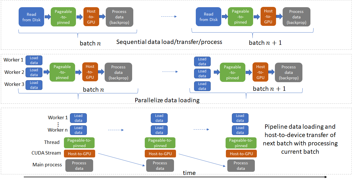
Each of these steps must be parallelized whenever possible and steps for the next batch should be pipelined with the current batch whenever no data dependencies exist.
Before I go further, quick note on the dataset and training code I’ll be using. I used the training imagenet example in Pytorch docs. Instead of the full Imagenet dataset, I used the tiny-imagenet dataset to keep the per epoch training time low. This dataset consists of 200 classes with 500 images each for training. Thus the number of images/epoch is ~10% of that of Imagenet.
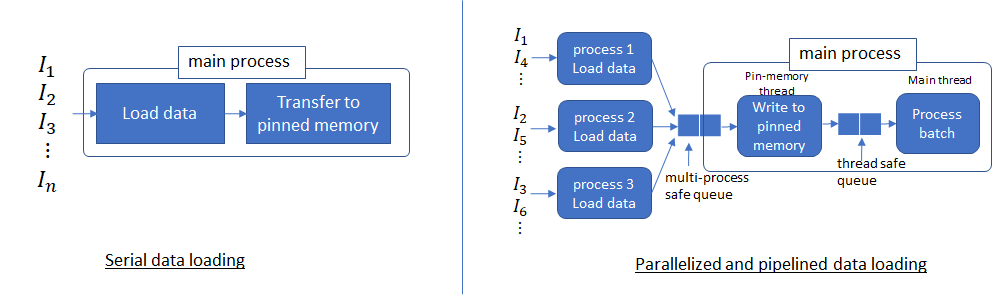
Fortunately, deep learning libraries provide support for all of these steps. Dataloader in Pytorch (the framework I’ll be focusing on in this post) provides the ability to use multiple processes (by setting num_workers > 0) to load data from the disk and multi-threaded data transfer from pageable to pinned memory (by setting pin_memory = True).

The plot below shows the data loading (red plot), host-to-device transfer (green plot) and processing (blue plot) times for Resnet 18 with a batch size of 256 on 1 1080 Ti GPU when num_threads = 0, meaning that data loading and data transfer are all done on the main thread with no parallelization.
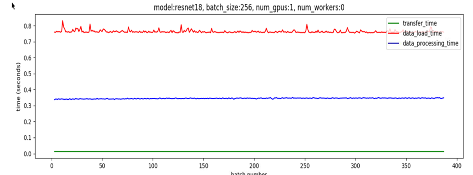
The data loading time dominates, which implies that no matter what we do to speed up data processing, performance will be limited by the data loading time. Now let’s set num_workers = 4 and pin_memory flag = True. By doing so, multiple processes are used to read non-overlapping data from the disk and a producer-consumer thread is spun up to transfer data read by these processes from pageable to pinned memory.
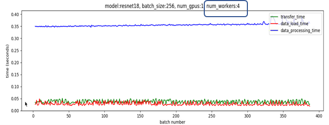
Now multiple processes are able to load data much faster and pipelined data loading can almost completely hide the data loading latency when the data processing time is long enough. This is because the data for the next batch is read from the disk and transferred to pinned memory in parallel with processing the current batch. If processing the current batch takes long enough, the data for the next batch is available immediately. This idea also suggests how to set an appropriate value for num_workers parameter. This parameter should be set such that batch data can be read from the disk quicker than the GPUs can process the current batch (but no higher, because that will simply waste system resources used by multiple processes).
Note that so far we have only addressed data loading from the disk and transfer from pageable to pinned memory. Data transfer from pinned memory to the GPU (tensor.cuda() ) can also be pipelined using CUDA streams. Pytorch’s default Imagenet example doesn’t do this, but NVIDIA’s apex library shows an example of how to do this. I’ll discuss this in more detail a bit later.
Data-parallel and distributed-data-parallel
We are now ready to examine data-parallel processing using a network of GPUs. The basic idea is that each GPU in the network runs the forward and backward pass on a batch of data using a local copy of the model. The gradients calculated during the backward pass are sent to a server which runs an reduce operation to compute averaged gradients. The averaged gradients are then transmitted back to the GPUs which update the model parameters using SGD. Using data parallelism and efficient network communication SW libraries such as NCCL, an almost linear reduction in training time can be achieved. There are lots of nice tutorials on the web that explain in great detail how data parallelism works. I also wrote a post last year that implements data parallelism on simulated data entirely in Python, without using any deep learning frameworks.
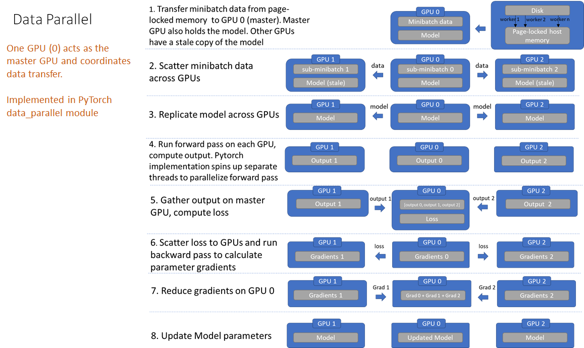
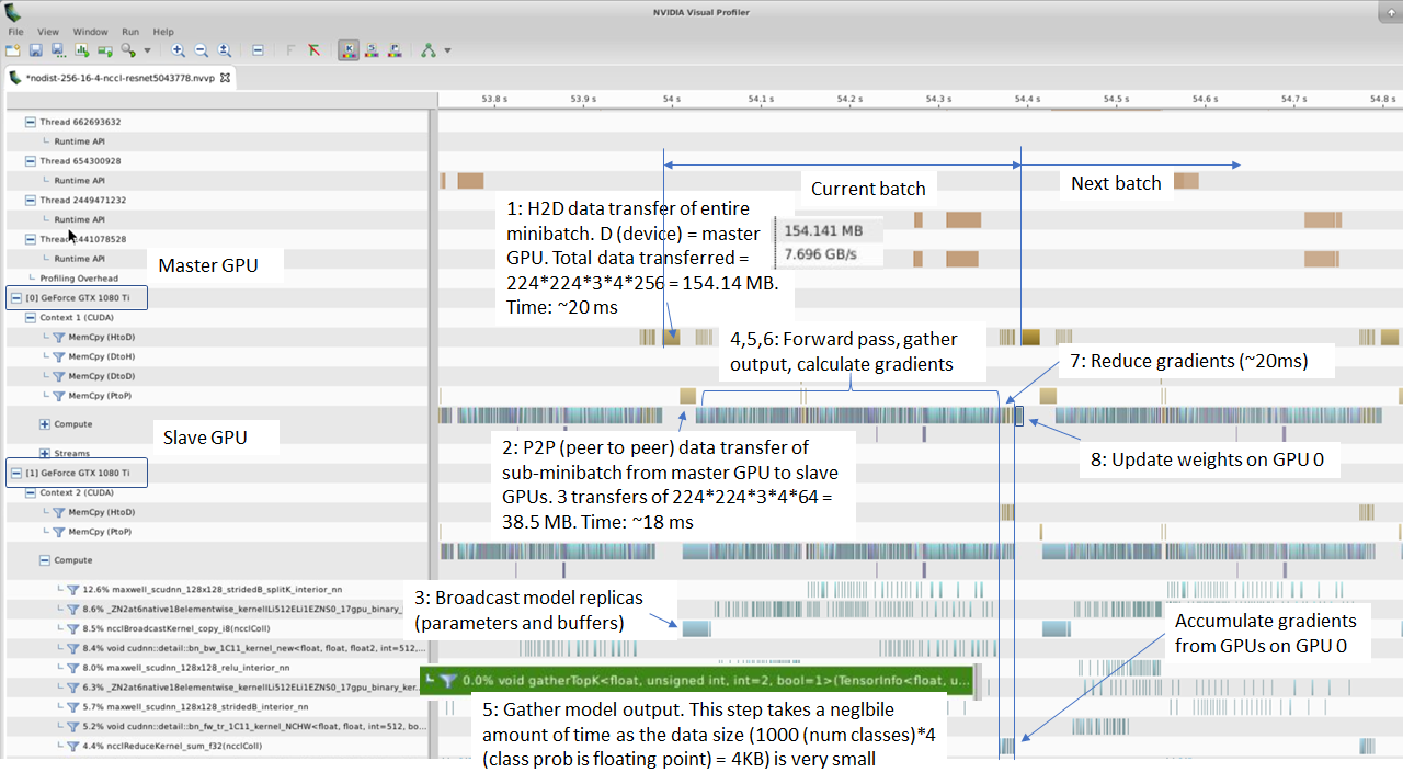
Pytorch 1.01 has two systems to support data parallelism. The first is implemented in nn.parallel.data_parallel and simply called data-parallel. As shown in the figures below, this system works by loading the entire mini-batch on the main thread and then scattering the sub mini-batches across the GPU network. Each GPU runs the forward pass on its sub mini-batch on a separate thread. The network outputs are then gathered on the master GPU and the loss function value is computed by comparing the network output with the true data labels for every element of the batch. Next, the loss value is scattered across the GPUs and each GPU runs the backward pass to compute gradients. Finally, the gradients are reduced on the master GPU and the model parameters on the master GPU are updated. This completes one iteration. Note that because the model parameters are only updated on the master GPU, the models on the other GPUs are now out of sync and model parameters must be broadcast to the other GPUs at the beginning of the next iteration.
You can follow along steps 2-5 in the forward function in nn.parallel.data_parallel.py. It is instructive to set up breakpoints in the Python code and inspect how data flows through each step.
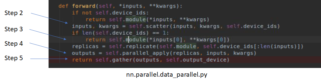
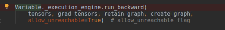
Unfortunately, the implementation of backward is hidden in C code, so you can’t step through the code in Python.
There are a number of inefficiencies in this design, as listed below.
- Redundant data copies
- Data is copied from host to master GPU and then sub-minibatches are scattered across other GPUs
- Model replication across GPUs before forward pass
- Since model parameters are updated on the master GPU, model must be re-synced at the beginning of every forward pass
- Thread creation/destruction overhead for each batch
- Parallel forward is implemented in multiple threads (this could just be a Pytorch issue)
- Gradient reduction pipelining opportunity left unexploited
- In Pytorch 1.01 data-parallel implementation, gradient reduction happens at the end of backward pass. I’ll discuss this in more detail in the distributed data parallel section.
- Unnecessary gather of model outputs on master GPU
- Uneven GPU utilization
- Loss calculation performed on master GPU
- Gradient reduction, parameter updates on master GPU
Using NVIDIA visual profiler
It is very instructive to use NVIDIA’s visual profiler (nvvp) to profile your Python application and visualize the results. I ran the Pytorch imagenet example on a system with 4 1080Ti GPUs for a few epochs.
|
1 |
$ nvprof -o profiler-output.nvvp python imagenet_data_parallel.py <location of dataset> --batch-size 256 --workers 4 --arch resnet50 |
I used the visual profiler to inspect the profiler output. A screenshot is shown below. I’ve marked each of the steps above so you can find them in the profiler output.
Using CUDA streams to pipeline host-to-GPU data transfers
I mentioned above that we haven’t exploited the opportunity to pipeline pinned memory-to-GPU data transfer. This can be accomplished using CUDA streams. If you are not familiar with CUDA streams, here’s an excellent tutorial from NVIDIA.
Let’s focus on the data loading and transfer portion from the profiler output above. A zoomed in version is shown below for convenience.
Notice that we are loading a batch of 64 images as FP32 values, this results in a total data size of 256  = 154.14 MB for a batch of 256
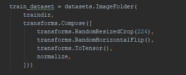
  images. Loading data as FP32 is clearly redundant as each pixel is represented as a 8 bit value. Next, this batch is split into 4 batches each with 64 images and scattered across the 3 GPUs. This operation can be pipelined with the data loading. Another operation that can be pipelined and performed on the GPU is normalization i.e, subtraction of mean and division by standard deviation of the image data. The default Pytorch Imagenet training implementation performs these steps after random resize and crop and random horizontal flip:
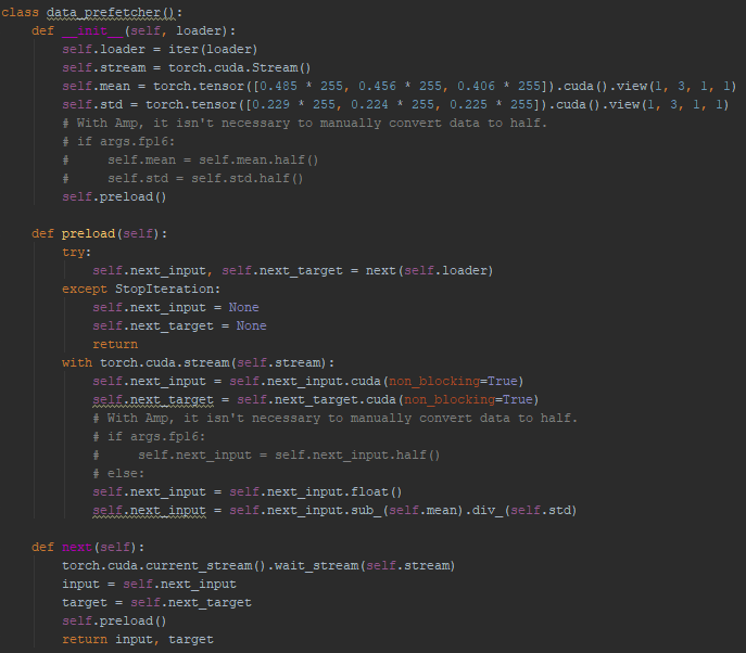
The NVIDIA APEX dataloader introduces a data_prefetcher class that fetches data from the Pytorch dataloader and uses CUDA streams to pipeline the data transfer to the GPU. The conversion to float and image normalization is now performed on the GPU, which is significantly faster than on the CPU and saves significant data loading bandwidth.
The table below shows timing results for running one epoch of training on tiny imagenet with and without pipelined host-to-GPU transfer and other optimizations in NVIDIA’s pre_fetcher on a 4 GPU system. The base case is running one epoch of training on one GPU, with the default data loader (no pre_fetcher). As you can see, using the pre_fetcher speeds up training by ~10%.
| Total Epoch Time (sec) | B (per GPU) | Num GPUs | Images/sec | Speed up | |
| Base case | 542 | 64 | 1 | 184.5 | 1x |
| Data Parallel (w/o streams) | 164 | 64 | 4 | 610 | 3.31x |
| Data Parallel (w streams) | 153.5 | 64 | 4 | 651.5 | 3.53x |
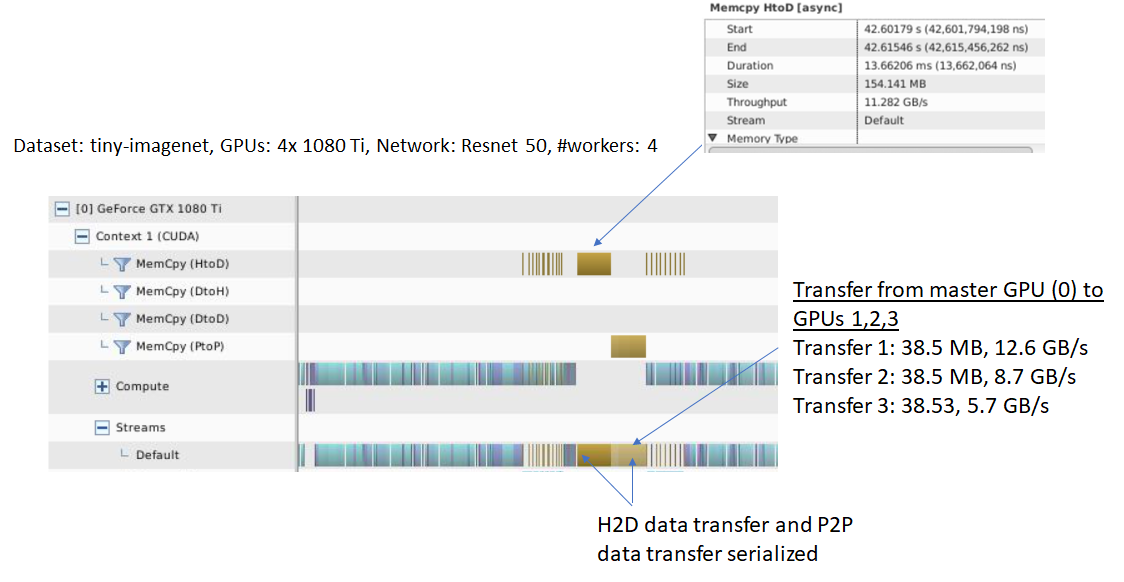
To finish this discussion, let’s look at the nvvp output with pre_fetcher optimizations.
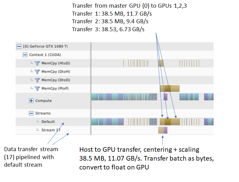
Now the amount of data read from the disk and transferred to the master GPU is 38.5 MB, one quarter the size before and occurs in its own stream, leaving the default stream free to do other tasks. Secondly, the transfers to the other 3 GPUs are also 1/4 smaller and pipelined with the host-to-device transfer. NVIDIA’s apex library introduces a number of other optimizations such as mixed precision training and dynamic loss scaling as well, which I did not investigate in these experiments. I took the code pertinent to the host-to-device pipelining and input normalization and added it to the Pytorch Imagenet example. The code can be downloaded here.
Distributed Data Parallel
Now, we are ready to look at the second system, distributed-data-parallel. The figure below shows the operation of distributed-data-parallel.
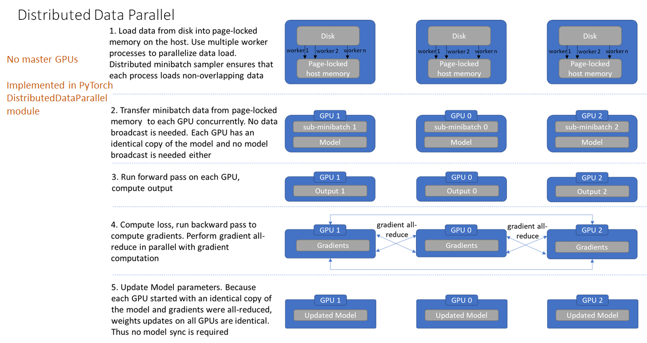
Distributed-data-parallel eliminates all of the inefficiencies noted above with data parallel. There is no master GPU anymore, each GPU performs identical tasks. Training on each GPU proceeds in its own process, in contrast with the multi-threaded architecture we saw earlier with data-parallel. Each process loads its own data from the disk. The distributed data sampler ensures that loaded data is non-overlapping across processes. We’ll examine how this works later. The forward pass and calculation of the loss function is executed independently on each GPU. Thus, no gathering of network outputs is required. During the backward pass, the gradients are all-reduced across the GPUs, ensuring that each GPU ends up with identical copy of the averaged gradients at the end of the backward pass. This design ensures that the updates to model parameters are identical, thereby eliminating the need for model syncs at the beginning of each iteration.
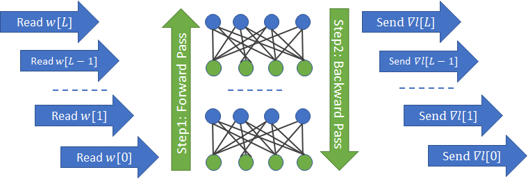
Besides its simpler data flow, distributed-data-parallel also takes advantage of another pipelining opportunity, gradient all-reduce with gradient computation. As shown below, calculation of parameter gradients for a layer has no dependency on the gradients of the previous layer. Thus gradient calculation in the backward pass can be pipelined with gradient all-reduce.
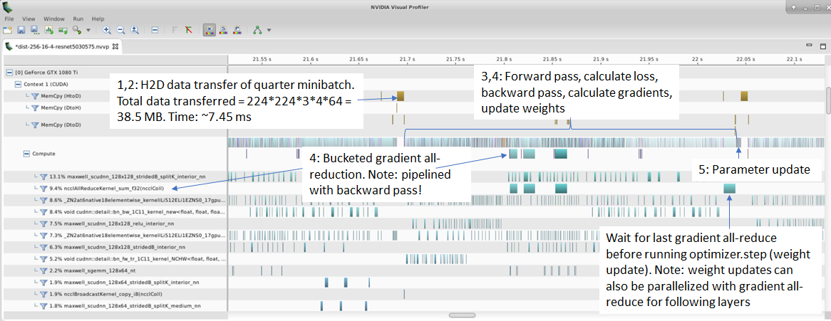
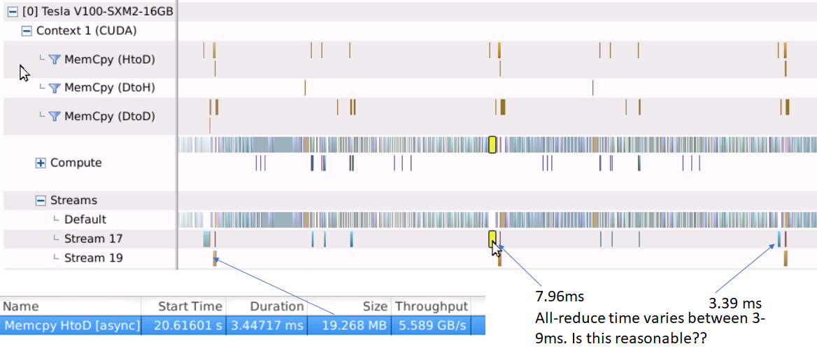
All of the steps shown above can be seen in the NVIDIA visual profiler output. This experiment was run without the optimizations in the apex library so the image data is still loaded as floating point values. The important thing to note is that the gradient all-reduce operations are neatly pipelined with the backward pass. Since gradients must first be calculated before they can be reduced, reduction must necessarily be one step behind the backward pass. Furthermore, to use network resources more efficiently, gradients are grouped into buckets before performing all-reduce. The default bucket size in Pytorch 1.01 is 25 MB. As shown below, the final weight update must wait for the last gradient all-reduce operation to finish.
|
1 2 |
$ nvprof -o profiler-output%p.nvvp --profile-child-processes python imagenet_distributed_data_parallel.py <location of dataset> --batch-size 256 --workers 16 --arch resnet50 --multiprocessing-distributed --world-size 1 --rank 0 --dist-url tcp://127.0.0.1:12345 |
The number of GPUs on the system is calculated automatically and a separate process is spawned to run training on each GPU. The number of workers processes used to load the image data is calculated by dividing the –workers argument above by the number of GPUs.
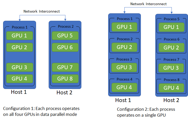
Distributed-data-parallel is typically used in a multi-host setting, where each host has multiple GPUs and the hosts are connected over a network. By default, one process operates on each GPU. According to Pytorch docs, this configuration is the most efficient way to use distributed-data-parallel. Another possible configuration is a single process running on each host that controls all the GPUs on that system. In this configuration, each process runs data-parallel (the first system we considered) on the GPUs it controls.
In a multi-host setting, the distributed-data-parallel application is launched on each host independently. Thus, some mechanism is needed so that the multiple processes running on separate hosts are in sync. This is the job of the init_process_group function that uses a shared file system or a TCP IP address/port to sync the processes.
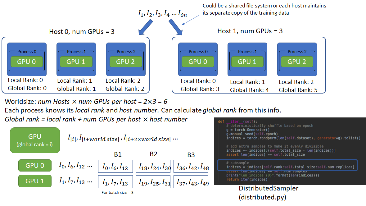
Another important requirement is that each process should load non-overlapping copies of the data. Pytorch provides a DistributedSampler that ensures this. Let’s consider a multi-host setting where one process controls one GPU. Lets say there are 2 hosts with 3 GPUs each. Each process can access the training data either via a shared file system or maintain its own local copy of the data. To read non-overlapping copies of the data, each process must know the number of processes in the process group and its own rank in the group. With this info, each process can use its rank as the offset and number of processes as the stride to read non-overlapping chunks. This information is provided through the parameters world_size and rank.
|
1 2 3 4 5 6 7 |
Host 1: $ python imagenet_distributed_data_parallel.py <location of dataset> --batch-size 256 --workers 16 --arch resnet50 --multiprocessing-distributed --world-size 2 --rank 0 --dist-url tcp://192.145.3.1:12345 Host 2: $ python imagenet_distributed_data_parallel.py <location of dataset> --batch-size 256 --workers 16 --arch resnet50 --multiprocessing-distributed --world-size 2 --rank 1 --dist-url tcp://192.145.3.1:12345 |
Here world_size refers to the number of hosts in the distributed system (2 in our example) and the rank is the rank of each host. From this info, the total number of processes is calculated as world_size  number of GPUs per host. This number (6 in our example) then becomes the new world_size. The global rank (unique among the process group) of each process is then calculated as local rank (GPU id) + number of GPUs per host host_rank. The global rank and the world size can serve as the offset and stride for each process to load non-overlapping batch data. I haven’t verified this, but I believe this setup requires the number of GPUs on each host to be the same.
Let’s now look at the timing results using distributed-data-parallel on 1 host with 4 1080Ti GPUs. The results also compare the performance of the NVIDIA Collective Communications Library (NCCL) and Gloo backends. As expected, the vendor provided communication backend has much better performance.
| Total Epoch Time (sec) | B (per GPU) |
Num GPUs |
Images/sec |
Speed up |
|
|
Base case |
542 | 64 | 1 | 184.5 | 1x |
|
Data Parallel (w/o streams) |
164 |
64 |
4 |
610 |
3.31x |
|
Data Parallel (w streams) |
153.5 |
64 |
4 | 651.5 |
3.53x |
|
DistributedDataParallel (streams, NCCL) |
140 |
64 |
4 | 714 |
3.88x |
|
DistributedDataParallel (streams, Gloo) |
166 |
64 |
4 | 602 |
3.27x
|
Distributed-data-parallel with NCCL backend achieves almost linear scaling!
So given that distributed-data-parallel appears to be simpler and faster than data-parallel, is there any reason to use data-parallel at all? I found data-parallel easier to debug. Since data-parallel runs in one process, it is easier to set breakpoints. Distributed-data-parallel being a multi-process system is more difficult to debug.
AWS Experiments
In this section, I’ll show how distributed training works on multi-GPU AWS servers and the impact of network BW on training time and scaling performance. I’ll also show what happens when there is a slow GPU server in the server mix.
I tested the following server configurations.
- 1 p3.8x instance (4 V100 GPUs)
- 2 p3.8x instances (8 V100 GPUs)
- 1 p3.16x instance (8 V100 GPUs)
- 3 p3.8x instances (12 V100 GPUs)
- 4 p3.8x instances (16 V100 GPUs)
- 2 p3.8x, 1 g3.16x – 8 V100, 4 M60 GPUs (12 fast and 4 slower GPUs)
Pytorch provides excellent instructions on how to set up distributed training on AWS. I first set up a single p3.8x instance with 4 GPUs and made sure I was able to run single host distributed-data-parallel. I then created an Amazon Machine Image (AMI) out of this instance and then launched other instances out of this image. Don’t forget the
|
1 |
export NCCL_SOCKET_IFNAME=ens3 |
part, as described in the instructions. Without this, distributed-data-parallel with NCCL won’t work. In the multi-host setting, make sure you set the world_size to the number of hosts (not GPUs). Also, the master host (whose IP you specify in –dist-url) must be rank 0. I simply launched the distributed training application manually on each host. The application will wait until all hosts have joined, so you don’t have to scramble to start the applications. You can also set up some orchestration script that launches the applications automatically.
One p3.8x instance
Let’s look at the timing results and the visual profiler output after running an epoch of training on one p3.8x instance.
|
Batch Size |
Num batches | Num GPUs |
Epoch time (sec) |
|
512 |
196 | 4 |
76.40 |
The total epoch time on the 4 V100 GPUs is much smaller than the 140 sec we saw earlier on the 4 1080Ti GPUs. We can also use a larger per GPU batch size (128 instead of 64). This makes sense as the V100 GPUs, designed for data center applications are a lot faster and have more memory than the consumer class 1080Ti GPUs.
The profiler output looks like this:
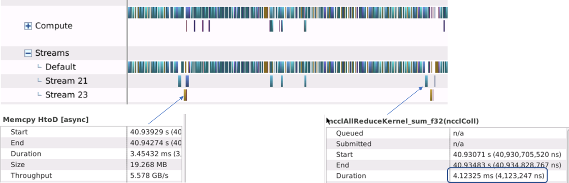
Like before, the gradient all-reduce operations are pipelined with the backward pass. The average all-reduce time (for a 25 MB bucket) is about 4 ms. It is instructive to calculate if this figure makes sense. Before we do this, let’s do a quick high level review of how all-reduce is implemented.
The all-reduce operation reduces the target arrays in all processes to a single array and replicates the resultant array to all processes. Reduction means an operation such as sum, mean etc., that is applied to corresponding elements of each target array. Let the number of array elements per process be and the number of processes be  . A naive all-reduce implementation selects one process as the master, gather all arrays into the master, perform reduction operations locally in the master, and then distributes the resulting array to the rest of the processes. Total data transferred (gather + scatter):
  . This is clearly not scalable, as data transferred scales with number of processes.
Fortunately, more efficient all-reduce algorithms exist. A popular one is called the ring algorithm. See this for a great description of how ring all-reduce works. The total data transferred during ring all-reduce is  , which is nearly independent of . The trade-off is that ring all-reduce involves
  data transfers, higher than the naive algorithm. This is also the reason why gradients are grouped together into buckets as we saw earlier. Even more efficient algorithms such as the recursive halving/doubling algorithm exist (used in Facebook’s training Imagenet in 1 hour paper), which only use
  data transfers, however for small server counts, the ring algorithm suffices.
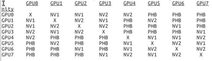
Once we know the total amount of data transferred, we can calculate the estimated time by dividing by the bandwidth of the slowest link in the all-reduce ring. For a multi-GPU system, the nvidia-smi utility can be used to see how the GPUs are connected with each other. On the p3.8x instance, running nvidia-smi topo -m produces:
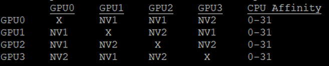
The bandwidth of the NVLink connections can be obtained by running nvidia-smi nvlink –status. The result is ~25 GB/sec. The expected all-reduce time is thus  = 1.5 ms, which seems to be in the right ballpark. The 25 in the numerator is the default size of the all-reduce bucket in Pytorch.
One p3.16x instance
Let’s now try the same experiment on a p3.16x server with 8 V100 GPUs. Timing and profiling results are shown below.
| Batch Size | Num batches | Num GPUs | Epoch time (sec) |
| 1024 | 98 | 8 | 37.6 |
The time to run one epoch is nearly one half of the time with 4 GPUs, which is good. The average all-reduce time for the last all-reduce bucket is ~4 ms. We can use the same procedure as before to figure out if this is reasonable.
Running nvidia-smi topo -m produces:
Here “PHB” stands for PCIe host bridge. With a BW of ~10 GB/sec, this is the slowest link in the all-reduce ring. The expected all-reduce time is thus  = 4.37 ms, which is in very good agreement with the observed time. In fact I suspect that in the case of 4 V100 GPUs that are interconnected over NVLinks, the PCIe host bridge is still in the loop somehow, which lowers the effective BW. It could also be that NV2 (meaning that the connection traverses two NVLinks) is twice as slow as NV1.
Two p3.8x instances
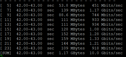
Now let’s consider two p3.8x instances connected over a 10 Gbit/sec internet connection. We can verify the actual link BW by running iperf3 (follow instructions here), which produces this output:
Profiling output and per epoch time looks like this:
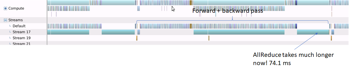
|
Batch Size |
Num batches | Num GPUs | Epoch time (sec) |
| 1024 | 98 | 8 |
45.6 |
The all-reduce operations now take much longer. The last all-reduce takes about 75 ms, which explains nearly all of the shortfall in linear scaling. With perfect linear scaling, epoch time = 76.4/2 = 38.2 sec. The observed time is 45.6 sec, 7.4 sec longer which is nearly equal to the delay caused by the last all-reduce (98 75 = 7.3 ms).
Multiple p3.8x instances
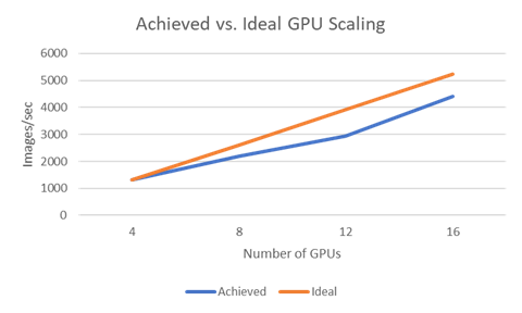
I also ran the same experiment on 3 and then 4 p3.8x instances. The timing results and scaling plot are shown below.
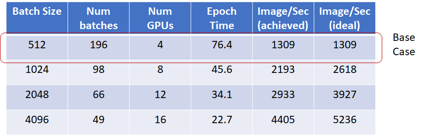
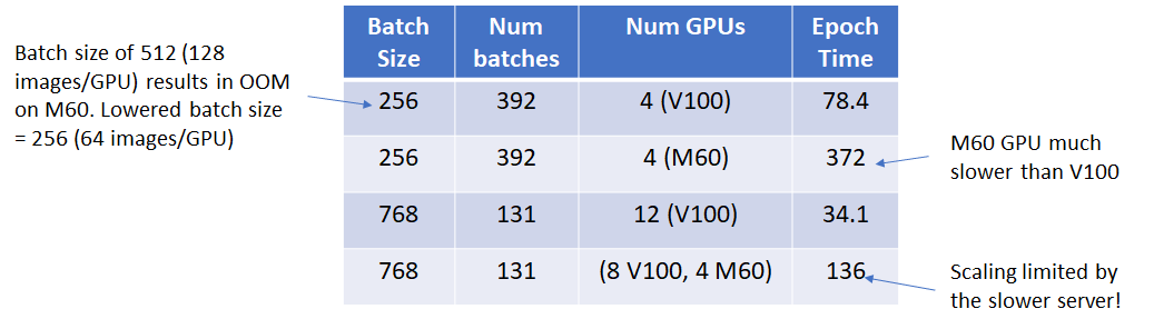
Adding a slower GPU server to the mix
Lastly, I wanted to see what happens if I throw in a slower GPU in the server mix. To test this, I used 2 p3.8x servers with 4 V100 GPUs each and one g3.16x server with slower M60 GPUs. The expectation is that the slower GPU will become the bottleneck for the entire system. As the results below show, this is indeed what happens!
Conclusion
In conclusion, using data parallelism is highly effective in leveraging multiple GPUs to scale DNN training. ML frameworks such as Pytorch provide built-in support for distributed training, but to use these features effectively, every data transfer and processing step must be well understood, parallelized and pipelined whenever possible. Among the two systems for data parallelism implemented in Pytorch 1.01, distributed-data-parallel is more efficient, but can be more difficult to debug.
The choice of collective communication backend can make a big difference in scaling performance. NCCL is faster than Gloo on a multi-GPU network.
Multi-GPU training using AWS GPU servers is easy to set up. Scaling performance is limited by the inter-server network BW. Also remember that the slowest GPU on the network will be the performance bottleneck, so ensure that your GPUs are equivalent in compute performance.
That’s it! Hope you found this information useful. Please leave a comment with your thoughts and feedback.
This is a very detailed resource, Excellent work, Ankur ! It is filled with precious insight and information. I think distributed training is a major topic that is not sufficiently discussed and documented. Thanks so much for sharing
Thanks Mehdi, glad you found the post useful.
I completely agree with Mehdi. I was having hard time following official documentation and not to mention dearth of tutorials. Your article made things a lot more clear. Thank you so much Ankur!
Glad you found it helpful. I also had a hard time understanding the difference between data parallel and distributed data parallel and figuring out how to profile them.. hence the post.
Amazing article, thanks a bunch and keep up the good work!
Thank you very much Ankur. It is an excellent work. You have filled lots of missing parts in my mind.
Extremely useful article. Thanks for sharing
Thank you for the detailed observations. This blog is highly informative, and at the same time easy to follow. I am going to use this as a guide for writing my own observations while training large models.
Thank you very much for the article, it surely gave much-needed clarity! Is it possible to access the source code?
I don’t have the source code for this project anymore.. sorry!
This really cool Ankur. Much of this is still relevant in 2025. I was able to replicate some of the experiments with pytorch memory profiler and have a write up here https://github.com/ajayrfhp/LearningDeepLearning/blob/main/distributed_training/benchmarking_experiments.MD.
It also includes links to scripts and notebooks that do the gpu training and benchmarking.