Neural Network Loss Visualization

Plotting its shape helps in understanding the properties and behaviour of a function. Unfortunately since we live in a 3D world, we can’t visualize functions of dimensions larger than 3. This means that using conventional visualization techniques, we can’t plot the loss function of Neural Networks (NNs) against the network parameters, which number in the millions for even moderate sized networks.

This NIPS 2018 paper introduces a method that makes it possible to visualize the loss landscape of high dimensional functions. I’ll briefly describe how the method works and refer you to the paper for details.

Training neural networks involves finding set of parameters that minimize a loss function . Here refers to the input, refers to the output data label and is the number of samples in the training batch. This minimization is typically performed using a variant of stochastic gradient descent. Let denote the final parameter values after training. Since can have millions of parameters, we can’t visualize the loss function against all the dimensions of . To visualize a slice of this loss function, we pick two random directions and with the same dimension as and plot the function against and . Here and are scalars that vary across a suitable range (such as ) on the and axis. The density of the plot is determined by the sampling step size.

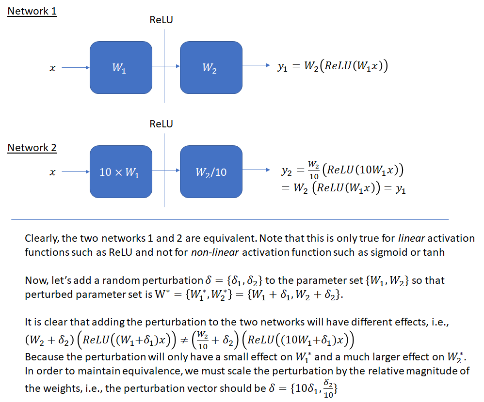
An important issue that must be kept in mind while making these plots is scale invariance. As shown below, the output of a network (with ReLU activation function) remains unchanged if we multiply the weights in one layer by a factor and divide the weights of the next layer by the same factor. This means that when the parameters of a networks are perturbed, the perturbation must factor the relative scale of the weights, otherwise a unit norm perturbation will affect a network with smaller magnitude weights more than a network with larger weights, even though the two networks may be equivalent. This will make the first network appear to have a sharper loss landscape, when this apparent sharpness is just a scale artifact. This invariance is even more prominent when batch normalization is used and the output of each layer is shifted and scaled according to the batch statistics. As mentioned in the original batch normalization paper,  , where BN denotes the batch normalization transformation and and are the weights and input for a layer.

The figure below illustrates the issue on a simple two layer fully connected network with the bias factor omitted. Please refer to the original paper for a more detailed explanation.

I have created a WebGL application to make it easy to visualize the loss landscape for some common neural networks. You can use the left/middle/right mouse button to rotate/zoom/pan the camera, turn wireframe mode on/off and overlay loss landscapes to make it easy to see differences between them. The differences are easier to see in wireframe mode as one is able to see through the loss landscape. On hovering over the loss landscape, a tooltip will show the x/y/z value of the loss function under the cursor position. A screenshot is shown below.

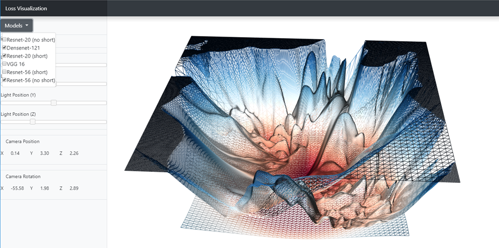
The application currently features the following models – Resnet-20 (short/no-short), Resnet-56 (short/no-short), Vgg 16 and DenseNet 121. As mentioned in the paper, the following observations can be made:

1. Effect of Network Depth: network depth has a dramatic effect on the loss surfaces of neural networks when skip connections are not used. The network Resnet-20 (no short) has a fairly benign landscape dominated by a region with convex contours in the center, and no dramatic non-convexity. However, as network depth increases, the loss surface of the VGG-like nets spontaneously transitions from (nearly) convex to chaotic. Resnet-56 (no short) has dramatic non-convexities and large regions where the gradient directions do not point towards the minimizer at the center
2. Shortcut connections prevent explosion of non-convexity: Shortcut connections have a dramatic effect on the geometry of the loss functions.  To recap, there are two main categories of networks that use shortcut connections
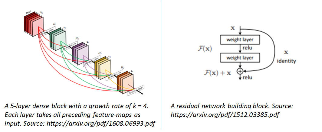
   1. Residual Networks: – These networks use residual building blocks where the input to some network blocks is added to the output of those blocks, making it possible for the block to learn the identity function. As shown in the original paper introducing residual networks, these residual connections enable training of extremely deep networks consisting of > 100 layers.
   2. Densely Connected Networks: In these networks,  (called DenseNet for short), each layer is connected to every other layer in a feed-forward fashion.

      

As networks get deeper, the loss landscape becomes increasingly gnarly (see landscapes for Resnet-20 (no short) and Resnet-56 (no short)). This makes the network sensitive to initial conditions and difficult to train. However residual connections prevent the explosion of non-convexity that occurs when networks get deep. Interestingly, the effect of skip connections seems to be most important for deep networks. See the difference between the loss landscapes of Resnet-56 (short) and Resnet-56 (no short). This effect seems to apply to skip connections used in DenseNet as well, whose loss landscape is very well behaved.

The loss landscape paper makes many other interesting observations – wide vs thin models, impact of network initialization and whether the dramatic dimensionality reduction done by this plotting procedure hides non-convexity that may be present in higher dimensions. The reassuring conclusion is that convex-looking regions in our surface plots do indeed correspond to regions with insignificant negative eigenvalues implying that there are no major non-convex features that the plot missed.