Initializing Weights for the Convolutional and Fully Connected Layers

You may have noticed that weights for convolutional and fully connected layers in a deep neural network (DNN) are initialized in a specific way. For example, the PyTorch code for initializing the weights for the ResNet networks (https://github.com/pytorch/vision/blob/master/torchvision/models/resnet.py) looks like this:

n = m.kernel_size[0] * m.kernel_size[1] * m.out_channels
m.weight.data.normal_(0, math.sqrt(2. / n))

1 2	n = m.kernel_size[0] * m.kernel_size[1] * m.out_channels m.weight.data.normal_(0, math.sqrt(2. / n))

The weights are initialized using a normal distribution with zero mean and standard deviation that is a function of the filter kernel dimensions. This is done to ensure that the variance of the output of a network layer stays bounded within reasonable limits instead of vanishing or exploding i.e., becoming very large. This initialization method is described in detail in the following paper by Kaiming He et al. (https://arxiv.org/pdf/1502.01852.pdf)

The purpose of this post is to provide some additional explanation, mathematical proofs, simulations results and explore additional topics such as adding bias and using rectifiers other than ReLU such as tanh and sigmoid. The post is organized as follows:

Section 1 – Implementing Convolution as Matrix Multiplication: You may notice that the same initialization method is used to initialize both fully connected and convolutional layers. Convolution and matrix multiplication are different mathematical operations and it’s not obvious how or why the same method can be used for both operations. In this section, we’ll show how this works.
Section 2 – Forward Pass (Without Bias): In this section, we’ll present a detailed proof of the variance propagation equations presented in He et al. paper and show some simulation results.
Section 2 – Forward Pass (With Bias): He et al. paper sets the bias to zero. In this section, we turn bias into a random variable and show how the parameters of the distribution from which bias is drawn should be set.
Section 4 – Other Rectifiers: In this section, we consider other commonly used rectifiers such as tanh and sigmoid functions.

Section 1: Implementing Convolutions as Matrix Multiplication

He et al. start their analysis of the propagation of variance during the forward pass with the following blurb:

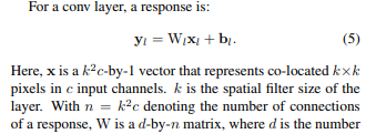
This immediately begs the question – convolution and matrix multiplication are different operations, how can matrix multiplication be used to implement convolutions? It turns out that by appropriately unfolding the input matrix (or the kernel matrix), convolutions can be implemented as a matrix multiplication.

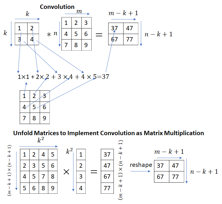
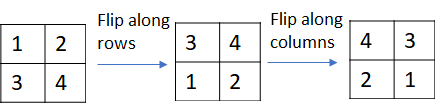
Strictly speaking, the calculation shown in the picture above implements correlation instead of convolution. Convolution can be implemented by simply flipping the kernel matrix along the rows and columns.

The python code to unfold an input matrix and implement correlation as a matrix multiplication is shown below

from scipy import signal
from scipy import misc
import numpy as np
from numpy import zeros

def unfold_matrix(X, k):
    n, m = X.shape[0:2]
    xx = zeros(((n - k + 1) * (m - k + 1), k**2))
    row_num = 0
    def make_row(x):
        return x.flatten()

    for i in range(n- k+ 1):
        for j in range(m - k + 1):
            #collect block of m*m elements and convert to row
            xx[row_num,:] = make_row(X[i:i+k, j:j+k])
            row_num = row_num + 1

    return xx

w = np.array([[1, 2, 3], [4, 5, 6], [-1, -2, -3]], np.float32)
#x = np.random.randn(5,5)
x = np.array([[-0.21556299, -0.11002319, -0.3499612,   1.49290769, -0.50435978],
 [ 0.06348409,  0.66873375,  0.14251138, -1.6414004 , -0.91561852],
 [-2.52451962, -1.97544675, -0.24609529, -1.11489934, -1.44793437],
 [ 1.26260575, -0.62047366,  0.12274525,  0.25200227, -0.83925847],
 [-1.54336488, -0.05100702,  0.36608208,  0.51712927, -0.97133877],
[-1.54336488, -0.05100702, 0.36608208, 0.51712927, -0.97133877]])

n, m = x.shape[0:2]
k = w.shape[0]

y = signal.correlate2d(x, w, mode='valid')

x_unfolded = unfold_matrix(x, k)
w_flat = w.flatten()
yy = np.matmul(x_unfolded, w_flat)
yy = yy.reshape((n-k+1, m-k+1))
print(yy)
# verify yy = y

from scipy import signal

from scipy import misc

import numpy as np

from numpy import zeros

def unfold_matrix(X, k):

n, m = X.shape[0:2]

xx = zeros(((n - k + 1) * (m - k + 1), k**2))

row_num = 0

def make_row(x):

return x.flatten()

for i in range(n- k+ 1):

for j in range(m - k + 1):

#collect block of m*m elements and convert to row

xx[row_num,:] = make_row(X[i:i+k, j:j+k])

row_num = row_num + 1

return xx

w = np.array([[1, 2, 3], [4, 5, 6], [-1, -2, -3]], np.float32)

#x = np.random.randn(5,5)

x = np.array([[-0.21556299, -0.11002319, -0.3499612, 1.49290769, -0.50435978],

[ 0.06348409, 0.66873375, 0.14251138, -1.6414004 , -0.91561852],

[-2.52451962, -1.97544675, -0.24609529, -1.11489934, -1.44793437],

[ 1.26260575, -0.62047366, 0.12274525, 0.25200227, -0.83925847],

[-1.54336488, -0.05100702, 0.36608208, 0.51712927, -0.97133877],

[-1.54336488, -0.05100702, 0.36608208, 0.51712927, -0.97133877]])

n, m = x.shape[0:2]

k = w.shape[0]

y = signal.correlate2d(x, w, mode='valid')

x_unfolded = unfold_matrix(x, k)

w_flat = w.flatten()

yy = np.matmul(x_unfolded, w_flat)

yy = yy.reshape((n-k+1, m-k+1))

print(yy)

# verify yy = y

We have only considered the case where the convolution kernel has one channel ( $c=1$ ). It is easy to see how the technique shown here can be generalized to more than one channel. In this case, the filter kernel matrix will be flattened to a $k^2c$ vector. There are a few other parameters related to convolution operation such as stride length and padding. For more information, see Karpathy’s post and also my post. In our example, stride length = 1 and padding = 0.

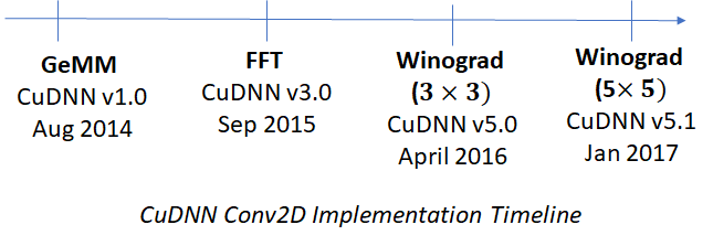
CuDNN v1.0 released in Aug 2014 used matrix multiplications to implement convolutions. This is computationally efficient because highly optimized libraries implementing matrix operations are already available. However conversion to matrix multiplication is not the most efficient way to implement convolutions, there are better methods available – for example Fast Fourier Transform (FFT) and the Winograd transformation. Generally speaking, FFT is more efficient for larger filter sizes and Winograd for smaller filter sizes ( $3\times3$ or $5\times5$ ). These implementations have become available in successive releases of CuDNN. A timeline is shown below.

Section 2: Forward Pass (without Bias)

Consider one layer of a neural network with input $\bf{x}$ , a $1\times n$ vector, weight matrix $\bf{W}$ , with dimensions $n\times m$ , output $\bf{a}$ – $1\times m$ vector which is a result of applying the ReLU activation function to the product of $\bf{x}$ and $\bf{W}$

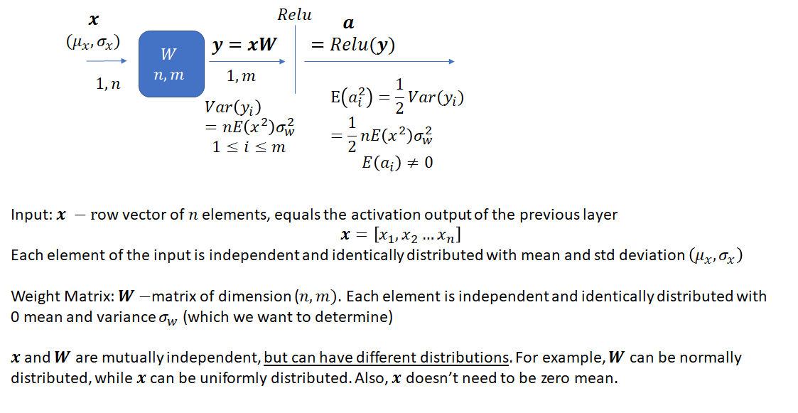
The task is to select an appropriate variance for the weights such that the variance of the network output stays bounded instead of vanishing or becoming excessively large, as the network gets deeper. As He et al. note, prior to the publication of their method, network weights were initialized using a Gaussian distribution with a fixed variance. With this approach, “deep” networks (networks with >8 layers) had difficulty converging. As an aside, it is interesting how “deep” neural networks have evolved in the last few years. The paper by He et al. was published in 2015 when a 8 layered network was considered deep. Now networks with 50 or even 100 layers are commonplace. He et al. noted that to avoid the vanishing/exploding gradient problem, the standard deviation of the weights must be a function of the filter dimensions and provided a theoretically sound mathematical framework (based on earlier work by Bengio and others). Their main conclusion can be summarized as follows:

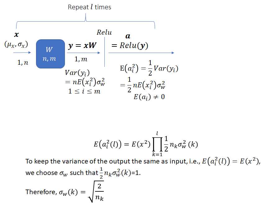
Notice that the standard deviation of the weights for a layer depends on the dimension of the layer. Thus, it is clear that for a network with multiple layers of different dimensions, a single choice for the standard deviation will not be optimal.

Let’s now consider the proof of the equations shown above and some simulation results.

Let’s first look at the proof for $Var(y_i) = nE(x_i^2)\sigma_w^2$ . Here, $x_i$ is an element of the input vector $\bf{x}$ .

(1) $\begin{equation*} y_i = ‎‎\sum_{k=1}^n ‎x_{k}w_{ik} \end{equation*}$

(2) $\begin{equation*}E(w_{ik}) = 0 \end{equation*}$

(3) $\begin{equation*} \begin{split} E(y_i) & = E(‎‎\sum_{k=1}^n x_{k}w_{ik}) \\ & = \sum_{k=1}^n E(x_{k}w_{ik}) \\ & = ‎‎\sum_{k=1}^n E(x_{k})E(w_{ik}) \text{ because } x_{k} \text{ and } w_{ik} \text{ are independent random variables} \\ & = 0 \text{ because } E(w_{ik}) = 0 \end{split} \end{equation*}$

Let’s first look at the covariances

(4) $\begin{equation*} \begin{split} Cov(y_i, y_j) & = E(y_i y_j) - E(y_i)E(y_j) \\ & = E(y_i y_j) \\ & = E(\sum_{k=1}^n ‎x_{k}w_{ik} \sum_{l=1}^n ‎x_{l}w_{jl}) \\ & = E(\sum_{k=1}^n ‎\sum_{l=1}^n w_{ik}x_{k} ‎x_{l}w_{jl}) \\ & = \sum_{k=1}^n ‎\sum_{l=1}^n E(w_{ik})E(x_{k}‎x_{l})E(w_{jl}) \\ & = 0 \end{split} \end{equation*}$

Now lets consider the variances

(5) $\begin{equation*} \begin{split} Var(y_i) & = Cov(y_i, y_i) \\ & = E(y_i^2)-E(y_i)^2 \\ & = E(\sum_{k=1}^n x_{k}w_{ik})^2 -E(y_i)^2 \\ & = E(\sum_{l=1}^n\sum_{k=1}^n x_{k}w_{ik}x_{l}w_{il}) \\ & = \sum_{l=1}^n\sum_{k=1}^n E(x_{k}w_{ik}x_{l}w_{il}) \\ & = \sum_{k=1}^n E(x^2_{k}w^2_{ik}) + \sum_{l=1}^n\sum_{k=1, k\neq l}^n E(x_{k}w_{ik}x_{l}w_{il}) \\ & = \sum_{k=1}^n E(x^2_{k})E(w^2_{ik}) \\ & = \sum_{k=1}^nE(‎x_{k}^2)(E(w_{ik}^2)-E(w_{ik})^2) \text{ since } E(w_{ik}) = 0 \\ & = nE(‎x_{k}^2)Var(w_{ik}) \end{split} \end{equation*}$

Here the last equality is due to the fact that $x_k$ and $w_{ik}$ are identically distributed. Note that $x_k$ and $w_{ik}$ need only be mutually independent, not identically distributed. To underscore this point, when we look at simulation results, we’ll draw $\bf{x}$ from a uniform distribution and $\bf{W}$ from a normal distribution.

Now, let’s look at the proof for $E(a_i^2) = \frac{1}{2}Var(y_i^2)$ for the ReLU activation function. Note that $Var(a_i) \neq E(a_i^2)$ because $E(a_i) \neq 0$ in general. However the cool part is that we don’t need the variance of $a_i$ to propagate the recurrence to the next network layer. $E(a_i^2)$ is all we need. In section 4, we’ll consider a general activation function of the form $a = \alpha y + \beta$ .

Dropping the subscript $i$ , $a = ReLU(y)$ , $\Rightarrow a = max(0, y)$ .

(6) $\begin{equation*} E[a^2] = \int_{-\infty}^{+\infty} \max(0,y)^2 p(y) dy \end{equation*}$

where the part $y<0$ does not contribute to the Integral

$\begin{align*} = \int_{0}^{+\infty} y^2 p(y) dy \end{align*}$

which we can write as half the integral over the entire real domain ( $y^2$ is symmetric around $0$ and $p(y)$ is assumed to be symmetric around $0$ ):

$\begin{align*} = \frac{1}{2}\int_{-\infty}^{+\infty} y^2 p(y) dy \end{align*}$

now subtracting zero in the square we get:

$\begin{align*} = \frac{1}{2}\int_{-\infty}^{+\infty} (y - E[y])^2 p(y) dy \end{align*}$

which is

$\begin{align*} = \frac{1}{2} E[(y - E[y])^2] = \frac{1}{2} Var[y] \end{align*}$

This completes the proof. Now let’s look at some simulation results which will validate the results presented here. Our simulation framework consists of a simple 10 layered network consisting of alternating layers of $5\times10$ and $10\times5$ weight matrices. Input is a $1\times5$ vector where each element is drawn from a uniform distribution (0,1). Thus, $E(x_i) = 0.5, Var(x_i) = 0.33$ . We’ll run the forward pass 100,000 times with randomly generated input and weights and look at the distribution of the network output. In each trial, the weights are drawn from a normal distribution with a mean and variance chosen using the method described here. The python implementation is shown below.

# number of layers
num_layers = 10

class layer(object):
    def __init__(self, _m, _n):
        #n: filter size (width)
        #m: filter size (height)
        self.m = _m
        self.n = _n
        self.activation = 'relu'
        #self.activation = 'tanh'
        #self.activation = 'sigmoid'

    def sigmoid(self, x):
        return 1 / (1 + np.exp(-x))

    def forward(self, x, use_bias = False):
       #x is a row vector
        self.W = np.random.normal(0, np.sqrt(2.0/self.m), (self.m,self.n))
        self.b = np.random.normal(0, np.sqrt(2.0/num_layers), self.n)
       # self.b = 1. - 2*np.random.rand(1, 5)
        self.y = np.dot(x, self.W)
        if (use_bias):
            self.y = self.y + self.b
        if (self.activation == 'relu'):
            self.a = np.maximum(0., self.y)
        if (self.activation == 'tanh'):
            self.a = np.tanh(self.y)
        if (self.activation == 'sigmoid'):
            self.a = self.sigmoid(self.y)
        return self.a, self.y


layers = []
# even numbered layers have a 5*10 weight matrix
# odd numbered layers have a 10*5 weight matrix
for i in range(num_layers):
    layers.append(layer(5 if(i % 2 == 0) else 10, 10 if(i % 2 == 0) else 5))

num_trials = 100000
# records the network output (activations of the last layer)
a = np.zeros((num_trials, 5))
# records the network input
i = np.zeros((num_trials, 5))
# record the activations
y = np.zeros((num_trials, 5))
for trial in range(0,num_trials):
    # input to the network is uniformly distributed numbers in (0,1). E(x) != 0.
    # Note that the distribution of the input is different from the distribution of the weights.
    x = 3*np.random.rand(1, 5)
    i[trial, :] = x
    for layer_no in range(0,num_layers):
        x, y_ = layers[layer_no].forward(x, False)
    a[trial, :] = x
    y[trial, :] = y_

#E(x^2) (expected value of the square of the input)
E_x2 = np.mean(np.multiply(i,i), 0)

# E(a^2) (expected value of the square of the activations of the last layer)
E_a2 = np.mean(np.multiply(a,a), 0)
# verify E_a2 ~ E_x2

# var(y): Variance of the output before applying activation function
Var_y = np.var(y,0)
# verify Var_y ~ 2*E_a2

# number of layers

num_layers = 10

class layer(object):

def __init__(self, _m, _n):

#n: filter size (width)

#m: filter size (height)

self.m = _m

self.n = _n

self.activation = 'relu'

#self.activation = 'tanh'

#self.activation = 'sigmoid'

def sigmoid(self, x):

return 1 / (1 + np.exp(-x))

def forward(self, x, use_bias = False):

#x is a row vector

self.W = np.random.normal(0, np.sqrt(2.0/self.m), (self.m,self.n))

self.b = np.random.normal(0, np.sqrt(2.0/num_layers), self.n)

# self.b = 1. - 2*np.random.rand(1, 5)

self.y = np.dot(x, self.W)

if (use_bias):

self.y = self.y + self.b

if (self.activation == 'relu'):

self.a = np.maximum(0., self.y)

if (self.activation == 'tanh'):

self.a = np.tanh(self.y)

if (self.activation == 'sigmoid'):

self.a = self.sigmoid(self.y)

return self.a, self.y

layers = []

# even numbered layers have a 5*10 weight matrix

# odd numbered layers have a 10*5 weight matrix

for i in range(num_layers):

layers.append(layer(5 if(i % 2 == 0) else 10, 10 if(i % 2 == 0) else 5))

num_trials = 100000

# records the network output (activations of the last layer)

a = np.zeros((num_trials, 5))

# records the network input

i = np.zeros((num_trials, 5))

# record the activations

y = np.zeros((num_trials, 5))

for trial in range(0,num_trials):

# input to the network is uniformly distributed numbers in (0,1). E(x) != 0.

# Note that the distribution of the input is different from the distribution of the weights.

x = 3*np.random.rand(1, 5)

i[trial, :] = x

for layer_no in range(0,num_layers):

x, y_ = layers[layer_no].forward(x, False)

a[trial, :] = x

y[trial, :] = y_

#E(x^2) (expected value of the square of the input)

E_x2 = np.mean(np.multiply(i,i), 0)

# E(a^2) (expected value of the square of the activations of the last layer)

E_a2 = np.mean(np.multiply(a,a), 0)

# verify E_a2 ~ E_x2

# var(y): Variance of the output before applying activation function

Var_y = np.var(y,0)

# verify Var_y ~ 2*E_a2

After running the simulation for 100,000 trials, $E(x^2), E(a^2)$ and $Var(y)$ are as follows:

$E(x^2)$ : [ 0.33347624 0.3329317 0.33355509 0.33261712 0.33284673]

$E(a^2)$ : [ 0.34210138 0.31643827 0.29113961 0.33775068 0.3297191 ]

$Var(y)$ : [ 0.7032769 0.64567238 0.61943556 0.66980425 0.65930914]

This agrees with the formulas presented earlier.

Section 3: Adding Bias

Let’s now consider the effect of adding a bias (which is a random variable instead of being initialized to 0) during the forward pass. Note that we haven’t performed any analysis on the effect of making the bias a random variable on network performance. The analysis presented here simply suggests a way to set the parameters of the distribution from which bias is drawn. Making the bias a random variable instead of setting it to zero may change the convergence properties of the network.

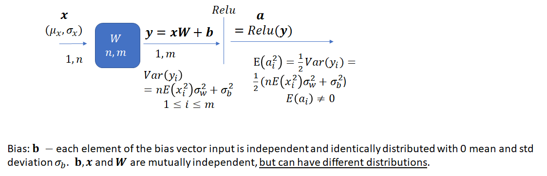
$Var(y_i)$ now has an additional term – the variance of the bias. Let’s first look at the proof and then consider how to select $\sigma_w$ and $\sigma_b$ such that variance of the network output remains bounded.

(7) $\begin{equation*} \begin{split} y_i = ‎‎&\sum_{k=1}^n x_{k}w_{ik} + b_i \\ E(y_i) = & E(‎‎\sum_{k=1}^n x_{k}w_{ik} + b_i) \\ & = \sum_{k=1}^n E(x_{k}w_{ik}) + E(b_i) \\ & = 0 \text{ because } E(w_{ik}) = 0 \text{ because } E(b_{i}) = 0 \end{split} \end{equation*}$

(8) $\begin{equation*} \begin{split} Var(y_i) & = Cov(y_i, y_i) \\ & = E(y_i^2)-E(y_i)^2 \\ & = E(\sum_{k=1}^n x_{k}w_{ik}+ b_i )^2 -E(y_i)^2 \\ & = E(\sum_{l=1}^n\sum_{k=1}^n (x_{k}w_{ik}+ b_i)(x_{l}w_{il}+ b_i ) \\ & = \sum_{l=1}^n\sum_{k=1}^n E((x_{k}w_{ik} + b_i)(x_{l}w_{il} + b_i)) \\ & = \sum_{k=1}^n E(x^2_{k}w^2_{ik} + b^2_i) \\ & = \sum_{k=1}^n E(x^2_{k})E(w^2_{ik}) + E(b^2_i) \\ & = nE(‎x_{k}^2)Var(w_{ik}) + Var(b^2_i) \text{ because } E(b_{i}) = 0 \end{split} \end{equation*}$

Choices for Weight and Bias Variances

We have the following recurrence equation for $E(a^2)$ in the presence of bias:

$E(a_i^2(l)) = \frac{1}{2}(n_l\sigma_w^2E(a_i^2(l-1))+\sigma_b^2)$

If we pick $\sigma_w = \frac{1}{\sqrt{n_l}}$ and $\sigma_b = 1$ , the recurrence equation becomes

$E(a_i^2(l)) = \frac{1}{2}(E(a_i^2(l-1))+1)$

Expanding the recurrence, we get the following expression for $E(a^2)$ after $k$ layers,

$E(a_i^2(l)) = \frac{E(x_i^2(l))}{2^k} + 1 - \frac{1}{2^k}$

This expression approaches 1 as the number of layers increases. This means that the effect of the input on the output diminishes as the network gets deeper. This is not the outcome we want. Let’s consider another choice for the variances. If we pick $\sigma_w = \sqrt\frac{2}{n_l}$ and $\sigma_b = \sqrt{\frac{2}{k}$ , then we get the following recurrence:

$E(a_i^2(l)) = E(a_i^2(l-1))+\frac{1}{k}$

Thus,

$E(a_i^2(k)) = E(x_i^2)+1$

This is a lot better. Now the output depends directly on the input and remains bounded. This result is also borne out through simulations. We make the following change to the code:

We initialize the weights and bias as follows:

self.W = np.random.normal(0, np.sqrt(2.0/self.m), (self.m,self.n))
self.b = np.random.normal(0, np.sqrt(2.0/num_layers), self.n)

1 2	self.W = np.random.normal(0, np.sqrt(2.0/self.m), (self.m,self.n)) self.b = np.random.normal(0, np.sqrt(2.0/num_layers), self.n)

While running the network, we set use_bias = True

for layer_no in range(0,num_layers):
    x, y_ = layers[layer_no].forward(x, True)

1 2	for layer_no in range(0,num_layers): x, y_ = layers[layer_no].forward(x, True)

After running the simulation for 100,000 trials, $E(x^2), E(a^2)$ and $Var(y)$ are as follows:

$E(x^2)$ : [ 0.33401292 0.33261908 0.33564588 0.33394963 0.33363114]

$E(a^2)$ : [ 1.36173389 1.42067756 1.34982683 1.4447972 1.31912953]

$Var(y)$ : [ 2.82221334 2.80030482 2.71711675 2.76212489 2.75131698]

What about the Backward Pass?

In our analysis so far, we have only considered the forward pass. It turns out that the initialization method doesn’t need to be modified when the backward pass is taken into account. This is because propagating gradients through fully connected and convolutional layers during the backward pass also results in matrix multiplications and convolutions, with slight different dimensions. For more details, refer to He et al. paper. Also, one of my posts about back-propagation through convolutional layers and this post are useful

Section 4: Other Activation Functions

So far, we have considered the ReLU activation function. ReLU has many desirable properties – it is mathematically simple, efficient to implement and leads to sparse activations. However, as shown in (https://arxiv.org/pdf/1602.05980.pdf), it is not too difficult to analyze the case for a more general activation function of the form $a = \alpha y + \beta$ . The recurrence is given as:

$var(y_i(l)) = n_l\alpha^2\sigma_w^2(var(y_i(l-1)) + \beta^2)$

Using Taylor series expansion, we can express many of the commonly used activation functions in the form $a = \alpha y + \beta$ . Let’s consider the taylor series expansion for sigmoid, tanh and ReLU activations.

$sigmoid(x) = \frac{1}{2} + \frac{x}{4} - \frac{x^3}{48} + O(x^5 ) \Rightarrow \alpha = \frac{1}{4}, \beta = \frac{1}{2}$

$tanh(x) = 0 + x - \frac{x^3}{3} + O(x^5 ) \Rightarrow \alpha = 1, \beta = 0$

$ReLU(x) = 0 + x \text{ for } x \ge 0 \Rightarrow \alpha = 1, \beta = 0$ .

Both tanh and ReLU activations have the desirable property that $\alpha = 1, \beta = 0$ and thus our initialization method will ensure that the variance of the output will lie in the proper range. However this is not true for the sigmoid function – first, $\alpha = \frac{1}{4}$ which means that the dependence of the output on the input will decrease as the network gets deeper, second, $\beta = \frac{1}{2}$ which makes the output gradient increase with each layer. I confirmed the first point in my simulation. Keeping the weight initialization method same as before (i.e, setting $\sigma_w^2 = \frac{2}{n_l}$ ), the variance of the output doesn’t change when I scale the input by a factor of 3. However, as pointed out in (https://arxiv.org/pdf/1602.05980.pdf), $\alpha \neq 1$ and $\beta \neq 0$ is not a fatal flaw. It can be corrected by rescaling the sigmoid activation function and adding a bias.

The key point to understand is the standard method to initialize weights by sampling a normal distribution with $\mu = 0$ and $\sigma_w^2 = \frac{2}{n_l}$ is not a “universally optimal ” method. It is designed for the ReLU activation function, works quite well for the tanh activation and not so well for sigmoid.

Telesens