

The purpose of this post is to provide some additional insights and Matlab and CNTK implementations for the two layer network used to classify a spiral dataset described in the following lecture of Stanford’s “Convolutional Neural Networks for Visual Recognition” class.
Using a neural network to classify a spiral dataset powerfully illustrates the effectiveness of NNs to handle inherently non-linear problems. It is evident that no linear classifier will be able to do a good job classifying spiral data where the boundary between two classes is a curve. A simple two layer network with RELU activation on the hidden layer automatically learns the decision boundaries and achieves a 99% classification accuracy on such a data set.
The problem description on the course website does a great job describing the problem, the architecture of the neural network used to solve it and the calculations in the forward and backward pass. This post makes the following contributions:
- Shows a movie of the decision boundaries as they are learnt by the network
- Provides Matlab and CNTK implementations for the Forward and Backwards pass (see appendix)
- Provides some additional insights related to variation of the classification accuracy with the number of hidden layer neurons, step size, and most importantly, the choice of the activation function
- Shows how to use custom loss and training functions in CNTK to achieve the same results as Matlab
Input Data
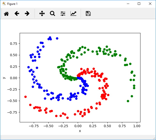
Our input data consists of 2D points (2 by 1 vectors) that are distributed along three spiral shaped arms. Clearly, a classifier with linear decision boundaries will be inadequate to classify such as dataset.
Movie Showing the Evolution of the Decision Boundaries
The movie shows the decision boundaries as they are learnt by the network. The boundaries start off linear but the network very quickly learns to bend them so they fit the contours of the data. This can be seen in the very sharp drop in the loss function in the beginning of the optimization.
You may be interested in the technique used to draw the decision boundaries and make the movie. For every “key frame” in the iteration, I ask the network to classify every point on the image frame (whose size is chosen to span our input data) by running the forward pass of the network. Each class is then drawn in a different color. The frequency of the “key frames” will depend upon how long you want the movie to be – if you have 2000 iterations and want the movie to be 6 seconds long playing at 15 FPS, you’ll need 90 frames. This means roughly 1 key frame every 20 iterations. The Matlab code to make the movie is included in the zip.
Variation of Classification Accuracy and Rate of Convergence with Step Size
The plots below show the loss curves for various step sizes in the Matlab implementation and the loss curve for Step Size = 1 using a Stochastic Gradient Descent learner for the CNTK implementation.
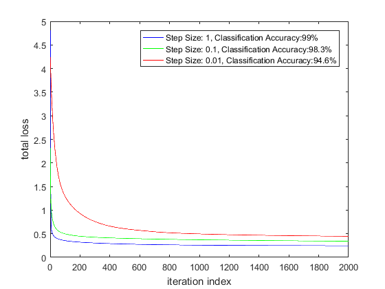
As expected, the loss function decays more slowly for lower step sizes. Somewhat surprisingly, the classification accuracy is slightly different for different step sizes. This could be because there are multiple local minimas at the bottom of the loss function valley. Since I’m using a constant step size during the optimization (instead of an adaptive technique where the step size is modified based on the first and second moment of the gradients), perhaps the optimization is achieving a slightly different minimum for different step sizes.
The plots below show the evolution of the loss function for the Matlab and CNTK implementation (left plot: Matlab, right plot: CNTK) for step size = 1.
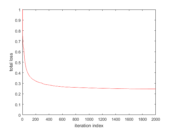
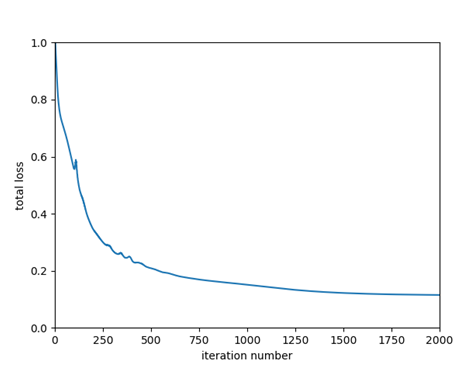
CNTK achieves a slightly lower total loss because the CNTK loss function comprises only of softmax with cross entropy component, not the L2 weight regularization component. Later, we’ll see how we can customize CNTK to use our loss function that adds the L2 regularization component to softmax with cross entropy. We’ll also replace CNTK’s Stochastic Gradient Descent implementation with our own.
| CNTK | Matlab | |
| Final Value of Loss Function | 0.1155 | 0.2462 |
Changing the Number of Neurons in the Hidden Layer
Next, let’s consider the effect of changing the number of neurons in the hidden layer. Classification accuracy for both the Matlab implementation and CNTK implementation is reported.
| Number of Neurons in Hidden Layer | Classification Accuracy (Matlab) | Classification Accuracy (CNTK) |
| 100 | 99% | 99% |
| 50 | 98.6% | 98.4% |
| 7 | 94.3% | 97.1% |
| 5 | 73.3% | 93.4% |
| 3 | 56.4% | 65.4% |
One can reduce the number of neurons in the hidden layer to 7 before the classification accuracy starts to drop significantly!
Classification Accuracy for Various Activation Functions
| Activation Function | RELU | Leaky RELU | Exponential RELU | Tanh | Sigmoid | None (Linear Activation) |
| Classification Accuracy | 98% | 98% | 94.7% | 97.3 | 89% | 49% |
We can see that activation functions with sharp changes such as RELU are the most effective. Among the non-linear functions, a centered function such as tanh is more effective than non-centered function such as sigmoid. Not using an activation function significantly degrades classification accuracy.
Using Custom Loss and Training Functions
CNTK provides built-in implementations for commonly used loss functions such as softmax with cross entropy and trainers such as Stochastic Gradient Descent, ADAM 1, ADAGRAD2 and some of their variants. However, some problems require implementing a custom loss and training function. CNTK’s implementation of softmax with cross entropy loss doesn’t include the contribution from weight regularization, although the gradient of the weight regularization is included in the gradient calculation and parameter update. As mentioned earlier, this is the reason why the final loss computed by CNTK is slightly lower than the loss computed by our Matlab implementation. One can ask CNTK to use a custom loss function as follows:
|
1 2 3 4 5 6 7 8 9 10 11 |
# Define our custom loss function def cross_entropy_with_softmax_plus_regularization(model, labels, l2_regularization_weight): w_norm = C.Constant(0); for p in (model.parameters): w_norm = C.plus(w_norm, 0.5*C.reduce_sum(C.square(p))) return C.reduce_log_sum_exp(model.output) - C.reduce_log_sum_exp(C.times_transpose(labels, model.output)) + l2_regularization_weight*w_norm my_loss = cross_entropy_with_softmax_plus_regularization(z, label, l2_regularization_weight) # plug-in our loss function into the trainer trainer = C.Trainer(z, (my_loss, eval_error), [learner]) |
Using this loss function, the final value of the total loss is very similar for the CNTK and Matlab implementations
| CNTK | Matlab | |
| Final Value of the Loss Function | 0.2540 | 0.2462 |
Similarly, you can also insert your own parameter update logic by defining a custom trainer, as follows:
|
1 2 3 4 5 6 7 8 9 10 11 12 13 |
def my_gradient_update(parameters, gradients): update_funcs = []; for p, g in zip(parameters, gradients): # ideally, these should be parameters.. don't know of a way to do this yet. learning_rate = 1; numSamples = 300; # we need to divide by numSamples as the gradients are not scaled by the mini-batch size. gradient_scale_factor = learning_rate/numSamples; update_funcs.append(C.assign(p, p - gradient_scale_factor * g)) return C.combine(update_funcs) learner = C.universal(my_gradient_update, z.parameters) trainer = C.Trainer(z, (my_loss, eval_error), [learner]) |
Appendix
Matlab Code:
CNTK Code:
Leave a Reply