

Over the last month, I have been exploring the world of deep learning. Deep learning based algorithms have been around for a long time, but have recently shot into prominence after many false starts. Researchers are able to apply these algorithms to solve many previously intractable problems in a range of areas such as image processing and natural language processing to achieve human-like performance. Much of this progress is a result of vast quantities of data now available to train these networks and the realization that graphical processing units (GPU) can be used to parallelize much of the computation involved in training deep networks.
Given the ability of deep learning networks to automatically deduce the structure of complex problems and the huge investment of money and brainpower being poured into the field by the tech industry, algorithms powered by deep learning will play an ever larger role in our lives. Thus, some knowledge of how deep learning works will become vital to people in a range of industries. Depending on your level of technical sophistication (and pain tolerance 🙂 ) there are many levels at which you can learn about deep learning. A non-technical person could benefit from understanding how performance of deep learning systems is measured, difference between rules based, supervised and un-supervised learning, how deep learning systems are trained and so on. A more technical person with some programming knowledge could install and play with one of the many deep learning libraries such as Caffe, Torch, TensorFlow, CNTK etc., that are available for free. If you are like me, you are not satisfied with understanding at a middling level. You want to understand how things *really* work. Fortunately, as I have discovered over the last month (and perhaps contrary to what you may have been led to believe), much of the mathematics that powers deep learning systems (particularly multilayered neural networks) is not that complex and within reach of someone with a college level knowledge of calculus and familiarity with matrix algebra and non-linear optimization techniques such as gradient descent. Understanding this math and implementing some model networks yourself will give you valuable insights on how neural networks work and the subtleties involved with training these networks and setting various hyper parameters.
At the most fundamental level, training a neural network is akin to solving a non-linear optimization problem where gradient descent is used to optimize parameters to minimize an objective function. I won’t go into details of how this is set up, as there are a number of excellent tutorials available on the web. I’ll point you to a few that I found particularly helpful.
- CNN’s for Visual Recognition (http://cs231n.github.io/) is excellent. Module 1 is particularly helpful. Read all parts of module 1, and make sure you follow how the minimal 2D toy data example works (I wrote Matlab code corresponding to the provided python code for the minimal 2D toy example during my own learning and will attach it to this post at some point).
- For Matlab implementation of the major deep learning algorithms (Convolutional Neural Networks, Auto Encoders, Deep Belief Networks etc), see https://github.com/rasmusbergpalm/DeepLearnToolbox. I can’t thank the author of this tool-box enough. Going through the code and following how neural networks are constructed, the final error is computed during the forward pass and how various gradients are calculated and propagated during the backwards pass was critical to get a solid understanding of deep learning systems.
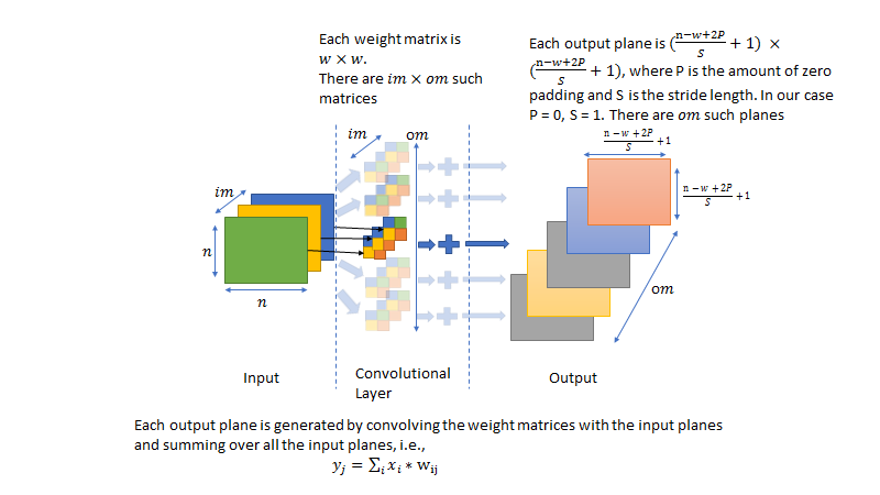
Training of neural networks proceeds by calculating the derivative of the output error wrt (with respect to) the input to a layer and the weights of that layer and then propagating the derivatives back through the preceding layers. The functional form of different operations applied in a layer (matrix multiply, sigmoid, pooling etc) are typically chosen so that calculating the derivatives is simple and efficient. The convolutional layers of a CNN are bit of an exception. There are many subtleties associated with how the derivatives wrt convolution filter weights are calculated and applied during gradient descent. The purpose of this post is to demystify how these derivatives are calculated and used. I’ll divide the post in two parts. In the first part, we’ll calculate the derivative of the output error wrt the weights analytically and compare the results with the gradient computed numerically. It will be gratifying to see that the two agree precisely. In the second post, we’ll consider a more realistic scenario where our input and output will consist of a batch of multi-dimensional planes and we’ll use gradient descent to calculate the optimal weights to minimize the error in the output for different values of a learning parameter. This process closely follows the calculation performed in a single convolutional layer of a real CNN.
The figures below demonstrate how the convolutional layer is structured and the notation used in the rest of this post. For clarity, it is good to keep track of the dimensions of various matrices during the forward and backward pass. To help the reader along, I specify the dimensions wherever applicable.
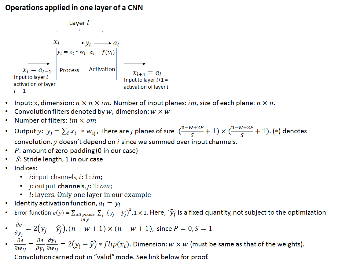
Note that I have stated without proof the rather remarkable result that the derivative of the error wrt weights of the convolution filter is the convolution of the flipped input and the output. For a detailed proof, please refer to:
http://jefkine.com/general/2016/09/05/backpropagation-in-convolutional-neural-networks/
This is an important result as the convolution operation can be efficiently implemented on GPUs. One could argue that if the derivative of the error had turned out to be some complicated expression that couldn’t be efficiently parallelized, many applications of deep learning in vision related applications may not be possible.
Part 1
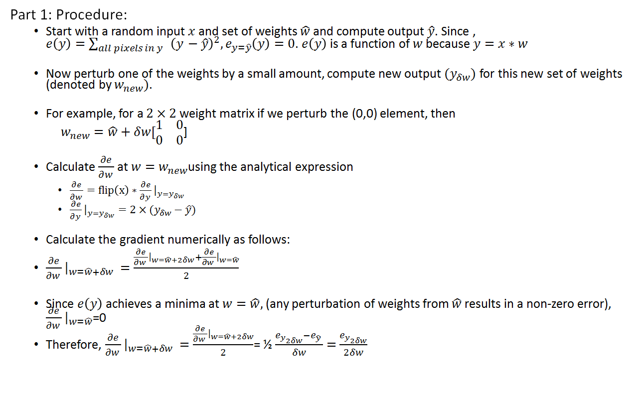
We’ll first consider a simplified example where the number of planes in the input and output is 1 and there is a single data sample in our batch. We’ll use the term “image” interchangeably with a data sample (underscoring the fact that the biggest application of CNNs is in image/vision processing). We’ll calculate the derivative of the error wrt filter weights using the analytical expression shown above and compare it with the derivative computed numerically. Doing so will clarify many of the subtleties involved with CNNs related to zero padding, output image dimensions, different convolution “modes” (full, valid) etc. The procedure and the matlab code is shown below. Note that we have dropped the input and output indicies ( ,
,  ) as the number of input and output planes is 1.
|
1 2 3 4 5 6 7 8 9 10 11 12 13 14 15 16 17 18 19 20 21 22 23 24 25 26 27 28 29 30 31 32 33 34 35 36 37 38 39 40 41 42 43 44 45 46 |
% Dimension of the input image is n*n n = 20; x = rand(n,n); % 3*3 Weight Matrix w = [1 2 3; 4 5 6; 2 3 4]; w_hat = w; % initial weights % Compute output, y is 18*18 y = convn(x, w_hat, 'valid'); y_hat = y; % Make a small change to the weights dw = 0.1; w = w + dw*[0 1 0; 0 0 0; 0 0 0]; % Calculate output using changed weights y_new = convn(x, w, 'valid'); % analytical derivative of error wrt y de_dy = 2*(y_new-y_hat); %18*18 % for derivation, see % http://jefkine.com/general/2016/09/05/backpropagation-in-convolutional-neural-networks/ % https://grzegorzgwardys.wordpress.com/2016/04/22/8/ de_dw_analytical = convn(flipall(x), de_dy, 'valid'); % Not required here, but for a multi-layered network, we'd also calculate % the derivative of the output wrt the input. This can be calculated by: de_dx_analytical = convn(flipall(w), de_dy, 'full'); % Note that we use convolution in "full" mode. This is because the size of % de_dx_analytical must match size of x % now calculate numerical derivative % output at w = w_hat + 2*delta_w w = w_hat + 2*dw*[0 1 0; 0 0 0; 0 0 0]; y_new2 = convn(x, w, 'valid'); ey_hat = sum(sum((y-y_hat).^2)); % 0 since y_hat is chosen to be y % error for the output at the changed weights ey_new = sum(sum((y_new2-y_hat).^2)); de_dw_numerical = (ey_new - ey_hat)/(2*dw); % verify that de_dw_numerical = de_dw_analytical function X = rot180(X) X = flipdim(flipdim(X, 1), 2); end function X=flipall(X) for i=1:ndims(X) X = flipdim(X,i); end end |
Part 2
Let’s now consider a more realistic scenario where we have a number of input and output planes and more than one data sample in our batch. Our initial estimate of the weights will be the true weight values with some added noise. We’ll run a gradient descent optimization to see if we can arrive at the correct weight values using the derivative of the output error wrt the weights calculated using the analytical expression and updating the weights in each iteration. We’ll apply a scale factor to the weight gradient before using it to update the weights. This scale factor will serve as our learning parameter. We’ll record the norm of the difference between the current weight values and the true values and plot the progression of this norm for different values of the learning parameter.
The Matlab code and the weight error plot is shown below.
|
1 2 3 4 5 6 7 8 9 10 11 12 13 14 15 16 17 18 19 20 21 22 23 24 25 26 27 28 29 30 31 32 33 34 35 36 37 38 39 40 41 42 43 44 45 46 47 48 49 50 51 52 53 54 55 56 57 58 59 60 61 62 63 64 65 66 67 68 69 70 71 72 73 74 75 76 77 78 79 80 81 82 83 84 85 86 87 88 89 90 91 92 93 94 95 96 97 98 99 100 101 102 103 104 105 106 107 108 109 110 111 112 113 114 115 116 117 118 119 120 121 122 123 124 125 126 127 128 129 130 131 132 133 134 135 136 137 138 139 140 141 142 143 144 145 146 147 148 149 150 151 152 153 154 155 156 157 158 159 160 161 162 163 164 165 166 167 168 169 170 171 172 173 174 175 176 177 178 179 180 181 182 183 184 185 186 187 188 189 |
% Note that I use a lot of for loops in this code and many of the for loops % can probably be more efficiently implemented as block matrix operations. % I feel that using block matrix operations can sometimes result in arcane % looking, hard to understand code. Since the point of this code is to % demonstrate how gradient descent for one layer of a CNN works, not to % show performant code, I haven't made any attempts to optimize performance. % dimension of input activation map (in each dimension). This can be % thought of as the "width/height" of an image n = 20; % number of input samples. This is equivalent to "Batch Size" nSamples = 10; % Filter size. Each filter is a square matrix of dimensions w*w % CNN's involve convolving input maps with rectangular (usually square) % filters that are a matrix of numbers, whose values we want to tune during % backpropagation. w = 2; % dimension of output activation map % As noted here http://cs231n.github.io/convolutional-networks/, the size % of the output image (along one dimension) = (n - w + 2P)/S + 1, % where S is the stride length (the amount in pixels by which we move the % weight matrix) and P is the amount of zero padding. In our case, the % stride length = 1, and no zero padding is used. Zero padding is generally % used if one desires the output activation map to have the same dimension as % the input activation map. S = 1; P = 0; m = (n - w + 2*P)/S + 1; % X: Input Data % Y: Output Data X = {}; % number of channels in the input/output activation maps. For images, % number of channels can be thought of as number of color planes. For gray % scale images, number of channels = 1, for RGB images, number of channels % = 3, for RGBA, number of channels = 4 and so on. im = 3; om = 5; % W indicates the weights matrix and Y the output cell matrix. underscore denotes % a running variable in the optimization. % W is cell matrix of dimension im*om. Each cell holds a single filter %(w*w matrix). Thus, there is a separate filter for each input % and output channel. The total number of weights for a filter of dimension % w, input channels: im, output channels: om = w*w*im*om. Same set % of weights is used for each input sample W = {}; W_ = {}; Y = {}; Y_ = {}; % Initialize the data. For each channel, we create n*n*nSamples % random numbers. If you think of input activation maps as images, % the data can also be thought of as nSamples of n*n images with im % channels for j = 1:im X{j} = rand(n,n, nSamples); end norm_dw = 0; % For each input and output channel, we initialize the filters to be a % w*w matrix of random numbers. We also add random noise to each % weight matrix. This will be the starting point of our gradient descent % optimization. The amount of noise is about 20% of the size of the % weights. for i = 1:im for j = 1:om, dW = rand(2,2); W{i}{j} = 5*rand(2,2); W{i}{j} = W{i}{j} - mean(mean(W{i}{j})); W_{i}{j} = W{i}{j} + dW; norm_dw = norm_dw + norm(dW); end end % calculate true output by convolving each channel of each input sample % with the weights for that channel and summing over the number of input % channels for j = 1:om % initialize each output channel to 0 z = zeros(m, m, nSamples); for i = 1:im, for x = 1: nSamples % Notice that output data for each input sample is stored % separately. We are not applying any averaging over input % images in a batch. % also note that each output is m*m z(:,:,x) = z(:,:,x) + conv2(X{i}(:,:,x), W{i}{j}, 'valid'); end end Y{j} = z/im; % j is the index of the output channel end % learning rate. Used later in the gradient descent iteration to scale the % computed derivative wrt the weights before updating the current estimate % of the weights. We'll run the optimization for three different values of % the learning rate and look at the rate of convergence steps = [1e-3, 3e-3, 5e-3] colors = ['r', 'g', 'b']; figure; for step_idx = 1: length(steps) numIter = 1; % array to hold the norm of dw (output error) and dw (difference between the true % weights and current estimate of the weights) norm_dw_arr = []; norm_dy_arr = []; % start off our initial estimates of the weights about 20% away from % the true weights for i = 1:im for j = 1:om, dW = rand(2,2); W_{i}{j} = W{i}{j} + dW; end end while numIter < 150 dY = {}; % Calculate output (Y_) using current estimate of the weights (W_) for j = 1:om % initialize each output channel to 0 z = zeros(m, m, nSamples); for i = 1:im, for x = 1: nSamples% for each image z(:,:,x) = z(:,:,x) + conv2(X{i}(:,:,x), W_{i}{j}, 'valid'); end end Y_{j} = z/im; dY{j} = Y_{j} - Y{j}; % size m*m end % calculate norm of the output error, although we won't be plotting % it here norm_dy = 0; for j = 1:om for s = 1: nSamples norm_dy = norm_dy + norm(dY{j}(:,:,s)); end end norm_dy = norm_dy/nSamples; norm_dy_arr(end+1) = norm_dy; %dX = convn(dY, rot180(W), 'full'); norm_dw = 0; % Let's now calculate derivative of error wrt the filter weights % using the analytical expression and run an iteration of gradient descent for j = 1:om, for i = 1:im, dW_analytical = zeros(size(W_{i}{j})); % calculate derivative of output wrt the filter weights. Note % that we sum over the number of samples. From a dimensionality % perspective, this makes sense as the dimension of dW must be % same as that of W. Each dW is a w*w matrix for x = 1: nSamples % backpropagate errors. Not used here, but would be % needed for a multi-layered network. dY_l = convn(dY{j}(:,:,x), flipall(W_{i}{j}), 'full'); % The flipping is essential. Without it, the derivatives % will be incorrect. dW_analytical = dW_analytical + conv2(flipall(X{i}(:,:,x)), dY{j}(:,:,x), 'valid'); end % Can also calculate dW_analytical by using a 3 dimensional % convolution, with the data samples being the third dimension % dW_analytical = convn(flipall(X{i}), dY{j}, 'valid'); % Average over nSamples dW_analytical = dW_analytical/nSamples; % Update current estimate of the weights W_{i}{j} = W_{i}{j} - steps(step_idx)*dW_analytical; norm_dw = norm_dw + norm(W_{i}{j} - W{i}{j}); end end norm_dw_arr(end+1) = norm_dw/(im*om); numIter = numIter + 1; end plot([1:numIter-1], norm_dw_arr, colors(step_idx)); hold on; end legend(['step size: 1e-3', 'step size: 3e-3', 'step size: 5e-3']) legend('step size: 1e-3', 'step size: 3e-3', 'step size: 5e-3') ylabel('norm of dw'); xlabel('iteration index'); function X = rot180(X) X = flipdim(flipdim(X, 1), 2); end function X=flipall(X) for i=1:ndims(X) X = flipdim(X,i); end end |
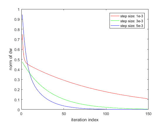
As we can see, the gradient descent is able to drive the norm of the weight error to nearly 0. As expected, the rate of convergence is higher for larger values of the learning rate. I haven’t shown it here, but too large a value of the learning rate causes the optimization to become unstable. Many methods are available to adjust the size of the learning rate during the gradient descent optimization as the change in the parameters during an iteration becomes smaller.
That’s it! Hope this post will help you better understand how gradients are calculated and used during backpropagation in a CNN.
Leave a Reply