Sensor Fusion: Part 1

In this series of posts, I’ll provide the mathematical derivations, implementation details and my own insights for the sensor fusion algorithm described in ¹. This paper describes a method to use an Extended Kalman Filter (EKF) to automatically determine the extrinsic calibration between a camera and an IMU. The underlying mathematics however can be used for a variety of applications such as performing sensor fusion between gyro and accelerometer data and using a camera to provide measurement updates to the gyro/accel sensor fusion. I will not be going into the theory behind Kalman filters. There is already a huge volume of publications that describe how Kalman filter work. Here are some references that I found useful.

Kalman and Bayesian Filters in Python². This is an excellent introductory reference and includes a number of practical examples along with code samples. It also provides a useful example of the math and code for implementing an extended Kalman filter.
Optimal State Estimation ³. This book is similar to the first reference, but provides many more examples and some new insights.
Stochastic Models, Estimation and Control ⁴. This book is the “bible” of estimation and control theory and a must read for serious practitioners in the field. It is however quite dry and can be very daunting for someone just getting started.
Indirect Kalman Filter for 3D Attitude Estimation⁵. This technical report provides a great introduction to matrix and quaternion math that we’ll be using extensively here.

Most references about Kalman filters that I came across either delve deep into the mathematics without providing a hands-on, practical insight into the operational aspects of the functioning of the filter or describe relatively trivial examples such as a position filter where everything is linear. For the EKF in particular, there are very few examples that illustrate how to calculate the Jacobians, set the covariance matrices and so on.

In this series of posts, we’ll first describe how to perform sensor fusion between accelerometer and gyroscope data and then add camera image measurements in the measurement update step. This problem is interesting to study from a mathematical and implementation standpoint and has numerous useful applications in vehicle navigation, AR/VR systems, object tracking and many others.

Let’s first quickly go over the basics of how a Kalman filter operates. Imagine you are standing at the entrance of a room and are asked to walk along a straight line into the room. This would be a trivial thing to do for most people; however to make things trickier, after you have taken a good look around the room, a blindfold is placed around your eyes. Let’s call the perpendicular distance to the straight line as your “state”. Since you start your journey from the origin of this straight line, your initial state and its “uncertainty” is zero. As you take each tentative step forward, guided by your sense of where the line is without actually being able to see it, the value of the state will change in a random manner. However the uncertainty in your state will always increase as with every step taken, you become increasingly uncertain of your position with respect to the straight line. The amount of increase in the uncertainty depends on the person – small for a tightrope walker and large for an inebriated person. The predict step in the Kalman filter models the act of taking a step in a mathematically precise way by using a set of matrices to model the transition from the current state (distance from the line before taking the step) to the next state (distance after the step is taken) and the amount of uncertainty injected in each step.

Now after you have taken a few steps and are quite uncertain about where you are with respect to the line, the blindfold is taken off and you are able to see your position with respect to the line. Now you can immediately adjust your state and are again quite certain about your position. This is the measurement update step in the Kalman filter. Measurements provide information about the state and help to reduce uncertainty. Measurements come with their own uncertainty and don’t have to provide direct information about the state. For example, your eye sight may not be perfect and you are still a little bit uncertain about your position or you may only be allowed to see around the room, but not directly at the floor where the line is. In this case, you’ll have to infer your position with respect to the line from your knowledge of the geometry of the room.

Let’s now make these ideas more concrete by putting them in mathematical language. The state $k$ is evolved from the state at $k-1$ according to

$\bf{x}_{k} = \bf{F}_k \bf{x}_{k-1} + \bf{B}_k \bf{u}_k + \bf{w}_k$

Here,

$\bf{F}_k$ is the state transition matrix. For simple problems, this matrix can be a constant, however for most real world applications, the transition matrix depends upon the value of the state vector and changes every iteration.
$\bf{B}_k$ is the control-input model which is applied to the control vector $\bf{u}$ . This can be used to model known control inputs to the system such as the current being applied to robot motors, the position of the steering wheel of a car etc. In our examples, we don’t assume any knowledge of control inputs, and thus $\bf{B}$ won’t be a part of our model.
$\bf{w}_k$ is the process noise which is assumed to be drawn from a zero mean multivariate normal distribution $\mathcal{N}$ , with covariance matrix $\bf{Q}_k: \bf{w}_k \sim \mathcal{N}\left(0, \bf{Q}_k\right)$ . Determining an appropriate value for this matrix can be tricky and often overlooked in literature on Kalman filters. I’ll describe my observations about how to set this matrix for the sensor fusion problem.

At time ”k” an observation (or measurement) $z_k$ of the true state is made according to

$\bf{z}_k = \bf{H}_k \bf{x}_k + \bf{v}_k$

where

$H_k$ is the observation model which maps state space into the observation space
$v_k$ is the observation noise which is assumed to be zero mean Gaussian with covariance $\bf{R}_k: \bf{v}_k \sim \mathcal{N}\left(0, \bf{R}_k\right)$

Note that $H_k$ maps the state vector to the observations, not the other way. This is because the $H_k$ is typically not invertible, i.e., it doesn’t provide direct visibility on the states.

The state of the filter is represented by two variables:

${\hat {\bf {x} }}_{k\mid k}$ , the a posteriori state estimate at time $k$ given observations up to and including that time;
$\bf{P}_{k\mid k}$ , the a posteriori error covariance matrix (a measure of the estimated accuracy of the state estimate).

The filter operates in two steps:

A predict step where the state and the covariance matrix is updated based on our knowledge of the system dynamics and error characteristics modeled by the $\bf{F}$ and $\bf{Q}$ matrices. The effect of the observations is not included in the predict step. This step is akin to taking a step with the blindfold on in our example described above.
A measurement update step where the effect of the observations is included to refine the state estimate and covariance matrix. This step is akin to taking the blindfold off in our example. Note that the predict and update steps don’t have to occur in lockstep. A number of predict steps could occur before an measurement update is made, for example the subject in our example could take several steps before the blindfold is removed. There could also be a number of different observations sources and the measurements from those sources can arrive at different times.

The corresponding equations for the predict and update steps are:

Predict

Predicted (a priori) state estimate	${\hat {\bf {x} }}_{k\mid k-1}=\bf {F} _{k}{\hat {\bf {x} }}_{k-1\mid k}$
Predicted (a priori) estimate covariance	$\bf {P} _{k\mid k-1}=\bf {F} _{k}\bf {P} _{k-1\mid k-1}\bf {F} _{k}^{T}+\bf {Q} _{k}$

Update

Innovation or measurement residual	${\tilde{\bf {y} }}_{k}=\bf {z} _{k}-\bf {H} _{k}{\hat {\bf {x} }}_{k\mid k-1}$
Innovation (or residual) covariance	$\bf {S} _{k}=\bf {H} _{k}\bf {P} _{k\mid k-1}\bf {H} _{k}^{\rm {T} }+\bf {R} _{k}$
Optimal Kalman gain	$\bf {K} _{k}=\bf {P} _{k\mid k-1}\bf {H} _{k}^{\rm {T} }\bf {S} _{k}^{-1}$
Updated (a posteriori) state estimate	${\hat {\mathbf {x} }}_{k\mid k}={\hat {\mathbf {x} }}_{k\mid k-1}+\mathbf {K} _{k}{\tilde {\mathbf {y} }}_{k}$
Updated (a posteriori) covariance	$\bf {P} _{k\|k}=(\bf {I} -\bf {K} _{k}\bf {H} _{k})\bf {P} _{k\|k-1}$

The main task in a Kalman filtering implementation is to use the system dynamics model and measurement model to come up with the state transition matrix $\bf{F}$ and measurement matrix $\bf{H}$ and the system noise characteristics to design the process and measurement noise covariance matrices.

Let’s now consider our specific problem. Our eventual goal is to derive equations 16 and 19 in ¹. To keep the math tractable, we’ll first consider a subset of the larger problem, i.e., how to combine the outputs of a gyroscope and accelerometer using a Kalman filter and later add the image measurements.

There exists a whole body of literature related to sensor fusion of inertial data. I will not go into the details here. Refer to DCMDraft2 for an excellent description of the relative strengths of a gyroscope and accelerometer and how to implement a complimentary filter to combine the data from these sensors.

The state vector in equation 16 consists of 21 elements.

$\delta{P_{I}^{G}}$ : Error in the position of the IMU in the global reference frame
$\delta{V_{I}^{G}}$ : Error in the velocity of the IMU in the global reference frame
${\delta\theta_{I}^{G}}$ : Error in the orientation between the IMU and the global reference frame
$\delta{P_{C}^{I}}$ : Error in the position of the camera with respect to the IMU
${\delta\theta_{C}^{I}}$ : Error in the orientation between the camera and the IMU
$\delta{b_{g}}$ : Error in gyro bias
$\delta{b_{a}}$ : Error accel bias

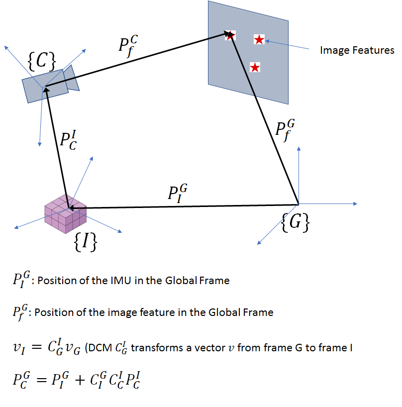
The three coordinate systems – global, IMU and camera frames are shown above. The notation used to describe position vectors and rotation matrices is shown above also. Let’s first consider a simpler problem – integrating the gyro data to produce orientation and using the accelerometer data as measurements to estimate the gyro bias and correct for drift. The state vector for this problem consists of 6 elements – the error in the orientation of the IMU with respect to the global frame of reference and the error in the gyro bias. Note that our state consists of errors in the orientation and gyro bias, not the orientation and the bias themselves. The reason for this choice will soon become clear.

In the discussion to follow, we’ll be evaluating the derivatives of vectors with respect to position and orientation repeatedly, so let’s establish a couple of vector differential calculus equations.

For a vector $v = [v_1 v_2 v_3]$ , the cross product skew symmetric matrix is defined as:

$[\bf{v}]_{\times} = \begin{bmatrix}0 & -v_3 & v_2 \\ v_3 & 0 & -v_1 \\ -v_2 & v_1 & 0\end{bmatrix}$ .

This matrix is called the cross product skew symmetric matrix because it can be used to express the cross product of two vectors as a matrix multiplication.

$\bf{a}\times\bf{b} = [\bf{a}]_{\times} \bf{b}$ .

This matrix is useful for us because it can use used to express the effect of a small rotation.

Let the orientation of a rotating frame B relative to a reference frame A at time $t$ be described by the DCM $C(t)$ and (equivalently) a quaternion $q(t)$ . Let the instantaneous angular velocity of B be given by $\boldface{\omega}$ . In a small time interval $dt$ , where this velocity can be assumed to be constant, the frame B would have rotated by $\phi = [\phi_x, \phi_y, \phi_z] = [\omega_xdt, \omega_ydt, \omega_zdt]$ along the axes of local coordinate frame to result in a new orientation at time $t+dt$ . Let’s consider using first DCM and then quaternions to represent this new orientation.

$C(t+1) = C(t)\exp(\phi_3)$

Here $\phi_3$ is a $3 \times 3$ skew symmetric matrix:

$\phi_3 = \begin{bmatrix}0 & -\phi_z & \phi_y \\ \phi_z & 0 &-\phi_x \\ -\phi_y & \phi_x & 0 \end{bmatrix}$ .

Expanding the exponential and using the properties of the skew symmetric matrix results in the well known rodrigues formula:

$C(t+1) = C(t)(I_3 + \frac{\sin(\theta)}{\theta}\phi_3 + \frac{1-\cos(\theta)}{\theta^2}\phi_3^2)$

here, $\theta = \sqrt{\phi_x^2 + \phi_y^2 + \phi_z^2}$ .

For small $\theta$ , rodrigues formula simplifies to:

$C(t+1) = C(t)(I_3 + \phi_3)$

Note that the multiplication with $\exp(\phi_3)$ above is a post multiplication instead of a pre-multiplication. This is because the small rotation represented by $\phi$ is applied in the body axis (the coordinate system obtained after applying $C(t)$ ). Using a pre-multiplication would result in the small rotation applied to the static (non-moving) reference frame.

Now let’s look at the quaternion representation. Using small angle representations, The quaternion representation for the small rotation $\phi$ is given as:

$\delta(q) \approx \begin{bmatrix}1 \\ \frac{\phi}{2} \end{bmatrix}$

At time $t+dt$ , the new orientation is given by the quaternion $q(t+dt)$ , where
$q(t+dt) = q(t)*\delta{q}$

In general, $\delta{q}$ will be a function of time (unless the body is rotating at a constant angular velocity).

$\frac{dq}{dt} = \lim_{\delta{t}\to 0}\frac{q(t)*[\delta{q}-I_q]}{\delta{t}}$

where $I_q$ is the identity quaternion. Substituting for $\delta{q}$ ,

$\dot{q} = \frac{1}{2}q(t)*\begin{bmatrix} 0 \\ \boldsymbol{\omega}\end{bmatrix}$

Using properties of quaternion multiplication, this expression can be written as a matrix product:
$\dot{q} = \frac{1}{2}[\omega_4][q]$

Here, $\omega_4$ is a $4\times4$ skew symmetric matrix, defined as (definition provided for $\phi_4$ )
$\phi_4 = \begin{bmatrix}0 & -\phi_x & -\phi_y & -\phi_z \\ \phi_x & 0 & \phi_z & -\phi_y \\ \phi_y & -\phi_z & 0 & \phi_x \\\phi_z & \phi_y & -\phi_x & 0 \end{bmatrix}$ .

Solving the differential equation,
$q(t+dt) = \exp(\frac{1}{2}\phi_4)q(t)$

Note that this solution automatically preserves the unit norm property of the new quaternion:
$q(t+dt)^Tq(t+dt) = q(t)^T\exp(-\frac{1}{2}\phi_4)\exp(\frac{1}{2}\phi_4)q(t) = q(t)^Tq(t) = 1$ since $\phi_4^T = -\phi_4$

Also, Using the properties of the $4\times4$ skew symmetric matrix, the quaternion representation can be simplified to:

$\exp(-\frac{1}{2}\phi_4) = I\cos(\theta) + \frac{1}{2}\phi_4\frac{\sin(\theta)}{\theta}$

Here, $\theta = \frac{\|\phi\|}{2}$

To avoid singularities associated with division by 0, a Taylor series expansion for $\frac{\sin(\theta)}{\theta}$ could be used.

to consolidate these ideas, let us look at some Matlab code to propagate the quaternion using the three methods described above.

function q_est = apply_small_rotation(phi, q_est)
s = norm(phi)/2;
x = 2*s;
phi4 = make_skew_symmetric_4(phi);
% approximation for sin(s)/s
sin_sbys_approx = 1-s^2/factorial(3) + s^4/factorial(5) - s^6/factorial(7);
exp_phi4 = eye(4)*cos(s) + 1/2*phi4*sin_sbys_approx;
% method 1
q_est1 = exp_phi4*q_est;
% verify: should be equal to:
% method 2 (direct matrix exponential)
q_est2 = expm(0.5*(phi4))*q_est;
% verify should be equal to:
% method 3: propagate by quaternion multiplication (doesn't preserve unit
% norm)
dq = [1 phi(1)/2 phi(2)/2 phi(3)/2];
dq_conj = [1 -phi(1)/2 -phi(2)/2 -phi(3)/2]';
q_est3 = quatmul(q_est, dq'); 
q_est = q_est1;
end


function phi4 = make_skew_symmetric_4(phi)
phi4 = [0       -phi(1)      -phi(2)      -phi(3);
    phi(1)     0           phi(3)     -phi(2);
    phi(2)     -phi(3)      0           phi(1);
    phi(3)     phi(2)     -phi(1)      0];
end

function q_est = apply_small_rotation(phi, q_est)

s = norm(phi)/2;

x = 2*s;

phi4 = make_skew_symmetric_4(phi);

% approximation for sin(s)/s

sin_sbys_approx = 1-s^2/factorial(3) + s^4/factorial(5) - s^6/factorial(7);

exp_phi4 = eye(4)*cos(s) + 1/2*phi4*sin_sbys_approx;

% method 1

q_est1 = exp_phi4*q_est;

% verify: should be equal to:

% method 2 (direct matrix exponential)

q_est2 = expm(0.5*(phi4))*q_est;

% verify should be equal to:

% method 3: propagate by quaternion multiplication (doesn't preserve unit

% norm)

dq = [1 phi(1)/2 phi(2)/2 phi(3)/2];

dq_conj = [1 -phi(1)/2 -phi(2)/2 -phi(3)/2]';

q_est3 = quatmul(q_est, dq');

q_est = q_est1;

end

function phi4 = make_skew_symmetric_4(phi)

phi4 = [0 -phi(1) -phi(2) -phi(3);

phi(1) 0 phi(3) -phi(2);

phi(2) -phi(3) 0 phi(1);

phi(3) phi(2) -phi(1) 0];

end

Either of these formulas can be used to propagate orientation. The quaternion representation is superior as it doesn’t suffer from singularities. Therefore, orientations should be maintained in quaternion form with other rotation representations extracted as needed.

Now let us consider the derivative of a vector rotated by a DCM $C$ with respect to position and small change in orientation. We’ll be using these derivatives repeatedly while formulating the EKF state propagation equations.

$\bf{v^{\prime}} = C\bf{v}$

derivative with respect to position:
$\bf{dv^{\prime}_v} = C(\bf{v+dv}- \bf{v}) = C\bf{dv}$

derivative with respect to orientation
$\bf{dv^{\prime}_\phi} = C(I_3 + \bf{d\phi_3})\bf{v}- C\bf{v} = C\bf{d\phi_3}\bf{v}$

Here $\bf{d\phi_3}$ is a $3 \times 3$ skew symmetric matrix of small rotations:

$\bf{d\phi_3}= \begin{bmatrix}0 & -d\phi_z & d\phi_y \\ d\phi_z & 0 &-d\phi_x \\ -d\phi_y & d\phi_x & 0 \end{bmatrix}$ .

Using the cross product notation,
$\bf{dv^{\prime}_\phi} = C[\bf{d\phi}]_\times\bf{v}$

For a cross product skew symmetric matrix, $[\bf{a}]_\times\bf{b}=-[\bf{b}]_\times\bf{a}$ . Hence,
$\bf{dv^{\prime}_\phi} = -C[\bf{v}]_\times\bf{d\phi}$

The nice thing about these expressions is that they allows us to express the derivatives wrt position and orientaion as matrix multiplications, which is required for the EKF state update and measurement update formulation.
$\begin{bmatrix}\bf{dv^{\prime}_v}, dv^{\prime}_\phi\end{bmatrix} = \begin{bmatrix} C & -C[\bf{v}]_\times \end{bmatrix}\begin{bmatrix}\bf{dv} \\ \bf{d\phi}\end{bmatrix}$

As an example, lets look at some Matlab code that implements the rotation and quaternion based updates.

% Original vector v
v = [1 1 1];
% Convert to unit vector
v = v./norm(v);
% Initial rotation (euler angles)
eul = [30 30 30]/57.3;
% Get quaternion and DCM representation for this rotation
q0 = eul2quat(30/57.3, 30/57.3, 30/57.3);
C0 = euler2dc(30/57.3, 30/57.3, 30/57.3);
% Apply rotation
v1 = C0*v';
% Small rotation (in radians)
phi = [0.01 0 0.01];
% Obtain the 3*3 and 4*4 skew symmetric matrices
phi3 = make_skew_symmetric_3(phi);
phi4 = make_skew_symmetric_4(phi);
s = norm(phi)/2;
x = norm(phi);
exp_phi4 = eye(4)*cos(s) - 1/2*phi4*sin(s)/s;
% Propagage quaternion
q1 = exp_phi4*q0';
% Propagate DCM (Rodrigues Formula)
C1 = C0*(eye(3) + sin(x)/x*phi3 + (1-cos(x))/x^2*phi3*phi3);
% Obtain the DCM corresponding to q1 to compare with C1
C_q1 = quat2dc(q1);
% Verify C_q1 ~ C1
% Now verify derivative wrt phi
% True value of the derivative
d1 = C1*v'-C0*v'
d2 = C0*make_skew_symmetric_3(v')*phi'
% verify d1 ~ d2

% Original vector v

v = [1 1 1];

% Convert to unit vector

v = v./norm(v);

% Initial rotation (euler angles)

eul = [30 30 30]/57.3;

% Get quaternion and DCM representation for this rotation

q0 = eul2quat(30/57.3, 30/57.3, 30/57.3);

C0 = euler2dc(30/57.3, 30/57.3, 30/57.3);

% Apply rotation

v1 = C0*v';

% Small rotation (in radians)

phi = [0.01 0 0.01];

% Obtain the 3*3 and 4*4 skew symmetric matrices

phi3 = make_skew_symmetric_3(phi);

phi4 = make_skew_symmetric_4(phi);

s = norm(phi)/2;

x = norm(phi);

exp_phi4 = eye(4)*cos(s) - 1/2*phi4*sin(s)/s;

% Propagage quaternion

q1 = exp_phi4*q0';

% Propagate DCM (Rodrigues Formula)

C1 = C0*(eye(3) + sin(x)/x*phi3 + (1-cos(x))/x^2*phi3*phi3);

% Obtain the DCM corresponding to q1 to compare with C1

C_q1 = quat2dc(q1);

% Verify C_q1 ~ C1

% Now verify derivative wrt phi

% True value of the derivative

d1 = C1*v'-C0*v'

d2 = C0*make_skew_symmetric_3(v')*phi'

% verify d1 ~ d2

I have not provided code for utility functions such as dcm to euler angle conversion. Any standard matrix algebra library can be used for implementation.

That is enough to digest for one post! In the next post, we’ll look at the EKF framework for performing gyro-accel sensor fusion.

Mirzaei FM, Roumeliotis SI. A Kalman Filter-Based Algorithm for IMU-Camera Calibration: Observability Analysis and Performance Evaluation. IEEE Transactions on Robotics. 2008;24(5):1143-1156. doi: 10.1109/tro.2008.2004486 [Source]

Labbe R. Kalman and Bayesian Filters in Python. Kalman and Bayesian Filters in Python. http://robotics.itee.uq.edu.au/~elec3004/2015/tutes/Kalman_and_Bayesian_Filters_in_Python.pdf. Published April 22, 2017.

Simon D. Optimal State Estimation. John Wiley & Sons, Inc.; 2006. doi: 10.1002/0470045345 [Source]

Maybeck P. Stochastic Models, Estimation and Control. Academic Press; 2012.

Indirect Kalman Filter for 3D Attitude Estimation. users.cs.umn.edu. http://www-users.cs.umn.edu/~trawny/Publications/Quaternions_3D.pdf. Published March 2005. Accessed April 23, 2017.

Simon D. Optimal State Estimation. John Wiley & Sons, Inc.; 2006. doi:10.1002/0470045345

Maybeck P. Stochastic Models, Estimation and Control. Academic Press; 2012.

Indirect Kalman Filter for 3D Attitude Estimation. users.cs.umn.edu. http://www-users.cs.umn.edu/~trawny/Publications/Quaternions_3D.pdf. Published March 2005. Accessed April 23, 2017.

Telesens

Sensor Fusion: Part 1

Predict

Update

Be the first to comment

Leave a Reply Cancel reply