

We are all familiar with GPS (Global Positioning System) and its myriad applications. From getting directions using Google maps to hailing a ride using a ride sharing app, countless individuals and businesses rely on accurate position estimation using GPS. Position estimation using GPS is now so accurate that GPS is being used for measuring plate tectonics and continental drift. Indeed, GPS is so much a part of our lives that few of us stop and wonder how it actually works. The purpose of this post is to show you how. More specifically, we’ll first learn how position is calculated from range measurements to GPS satellites and then consider a concrete example where we’ll process raw data collected by a commercial GPS receiver to obtain user position estimates.
GPS is owned by the US government and operated by the US air force. As such, access to GPS data can be degraded or denied to other nations due to geopolitical concerns. For example, according to this wikipedia article, access to GPS data was denied to the Indian military during the Kargil conflict. Other countries therefore decided to implement their own GPS like systems. Examples are GLONASS by Russia, Galileo by the European Union and BeiDou by China. This may seem like a waste of resources, but many of these systems operate using the same standards as GPS and are interoperable. For example, latest GPS receivers can receive signals from both GPS and GLONASS satellites, improving positioning accuracy. The wikipedia article referenced above also provides an interesting history of the origins of the GPS system dating back to Sputnik, the first man made satellite launched in space.
The post is divided into 3 parts – the first part describes the various coordinate systems used to express position. An understanding of these coordinate systems is essential for understanding how GPS works and is useful in its own right. For example, the concept of height above the earth surface is something that people intuitively understand, but turns out to be tricky idea to precisely define. The second part describes the basic principle of triangulation used by GPS to calculate position and develops the mathematics for calculating the user position from satellite measurements. A casual user, interested in a general knowledge of how GPS operates but not in the details can read part 1 and the first few sections of part 2 before the math starts. Finally, the appendix provides the Matlab code for implementing various ideas discussed in this post.
Most of the information in this post derives from the book “Global Positioning Systems: Signals, Measurements and Performance” 1, an excellent book about GPS systems. The matlab code presented in this post was written as solutions to the various end of chapter problems in the book. I also make use of material in the GPS Interface Specification document2. My contribution is to present the keys ideas related to GPS in a (hopefully) clear and concise manner and show the Matlab code that implements the positioning algorithms on real world data collected using commercial GPS receivers that can be purchased from the internet. After reading this post, a casual reader should have a better understanding of GPS, so the next time they use Google maps on their phone, they are aware of the amazing technical infrastructure that makes positioning and navigation applications possible. A more technical reader should be able to replicate my experiments by collecting their own data and running the Matlab code.
Table of Contents
Part 1
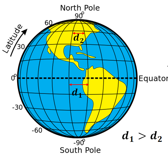
The fundamental task of a GPS system is to calculate position. To do so, we must first define what position means. Most people think about latitude/longitude and height when they think about position. While latitude/longitude are useful to represent a position on the earth surface, they are not suitable for mathematical calculations as they don’t provide a cartesian coordinate system. The physical distance represented by a unit difference between two longitudes is not constant, and depends on the position. For example, the distance between two longitudes one degree apart is greatest at the equator and approaches 0 at the poles.
To be useful for mathematical calculations, a coordinate system where a unit difference between coordinates represents a constant physical distance is required. A family of such coordinate systems can be created by defining a set of perpendicular axes intersecting at an origin that is rigidly attached to the earth. Such coordinate systems are called “ECEF” (Earth Centered, Earth Fixed). These coordinate systems work well to express the position of a user on earth as they rotate with the earth and the position of a stationary user on the earth surface is constant.
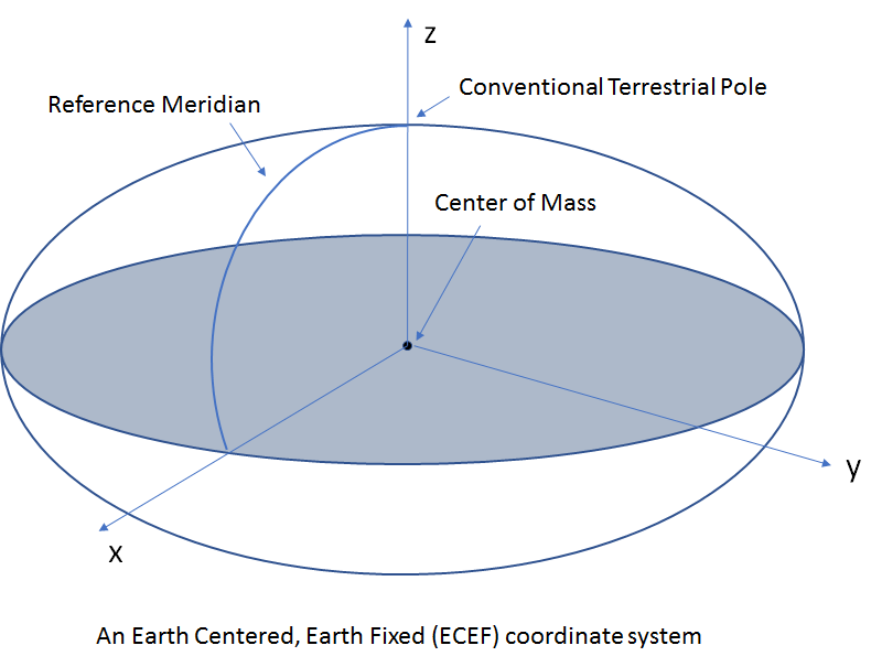
The most commonly used ECEF coordinate system is called the WGS 1984 system developed by the department of defense. WGS 84 is an ECEF frame, defined as follows:
- Origin at the center of mass of the earth
- z axis passing through the CTP (Conventional Terrestrial Pole). CTP is the average of the earth’s pole’s position between the years 1900 and 1905. An average needs to be used as the position of the pole is not fixed and wanders around in a circle of radius ~15m.
- x axis passing through the intersection of the CTP’s equatorial plane and a reference meridian, often called the Mean Greenwich Meridian
ECEF frames are convenient to represent positions with respect to the earth, but they are not inertial as they are rigidly attached to a spinning earth. To formulate the problem of satellite motion around the earth in accordance with Newton’s laws of motion, we need an inertial coordinate system in which to express acceleration, position and velocity vectors.
An inertial frame can be defined in a manner similar to the ECEF frame except that the x-axis points to the vernal equinox (the direction of intersection of the equatorial plane of the earth with the plane of the earth’s orbit around the sun). Strictly speaking, this frame isn’t inertial either since the earth is moving around the sun. However, it can be considered inertial over short periods (just as the ECEF frame can be considered inertial for analyzing the movement of a body on earth over a short period).
In the rest of this post, we’ll be using the WGS 84 ECEF frame to express the user and satellite position. This is possible because the GPS interface specification document (referred to as GPS-IS in the rest of this post) provides a step by step procedure to calculate the satellite position in the ECEF frame at a given time instant that accounts for the non-inertial nature of the ECEF frame. This is fortunate because ECEF frames are ideal to express the position of a user on the surface of the earth as they rotate with the earth and thus the position of a stationary user is constant, as one would expect. This would not be the case if an inertial reference frame is used to express position as such a frame would be fixed in space, and thus would appear rotating with respect to the earth.
Let’s now turn to the issue of defining height that we alluded to earlier. The key question that needs to be answered when defining height is “with respect to what”? Consider for example the height of a point in a desert. If we define height to be the distance of the point from the “ground”, then such a height would change constantly as the level of the ground itself changes due to natural phenomenon (for example, the wind depositing more sand). Thus, to define height, we must first define “ground” (note that strictly speaking, this issue doesn’t arise in a ECEF reference frame, as all distances are measured with respect to the center of mass of the earth. However generally people are not interested in distance from the center of the earth, but from the local earth surface). To define “ground” in a consistent manner, we need a model for the surface of the earth. Two models are generally used:
Model 1: Reference Ellipsoid
The surface of the earth is modeled as an oblate ellipse called the “reference ellipsoid”, centered at the earth’s center with the axis of revolution coincident with the z axis of an ECEF frame. The lengths of the semi-major and semi-minor axes (denoted as  and
and  ) are
) are  and
and  . As expected, the value generally used for earth’s radius (with the earth modeled as a sphere) is 6371Km which lies between the lengths of the semi-major and minor-axis. The reference ellipsoid is merely an abstraction for the shape of the earth. It doesn’t have any physical significance. An actual point on the earth surface will usually lie above or below the reference ellipsoid.
Model 2: Geoid
Another surface commonly used to measure height that does have physical significance is called the geoid. This surface is defined as the locus of all points with the same value of the gravitational potential. If the earth was a sphere with a uniform composition, this surface would be a regular surface that can be parameterized as a mathematical function. However since the earth is neither spherical nor uniform, the geoid is usually specified as a series of heights above the reference ellipsoid. Height relative to the geoid is called the orthometric height, or height above the mean sea level (MSL). This makes sense as if the oceans covered the surface of the earth, the shape of the oceans would be a close approximation to the geoid. Strictly speaking, the shape of the geoid itself is not fixed as the surface of the earth is constantly changing due to human activities and natural phenomenon. However given the bulk of the earth, these only have a negligible impact on the earth’s gravitational field and thus on the shape of the geoid.
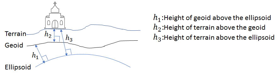
Note that the height of the geoid is specified with respect to the reference ellipsoid and the height of a given point can be specified with respect to either. The relationship between the ellipsoid, geoid and the actual surface of the earth is shown below.
Latitude and Longitude
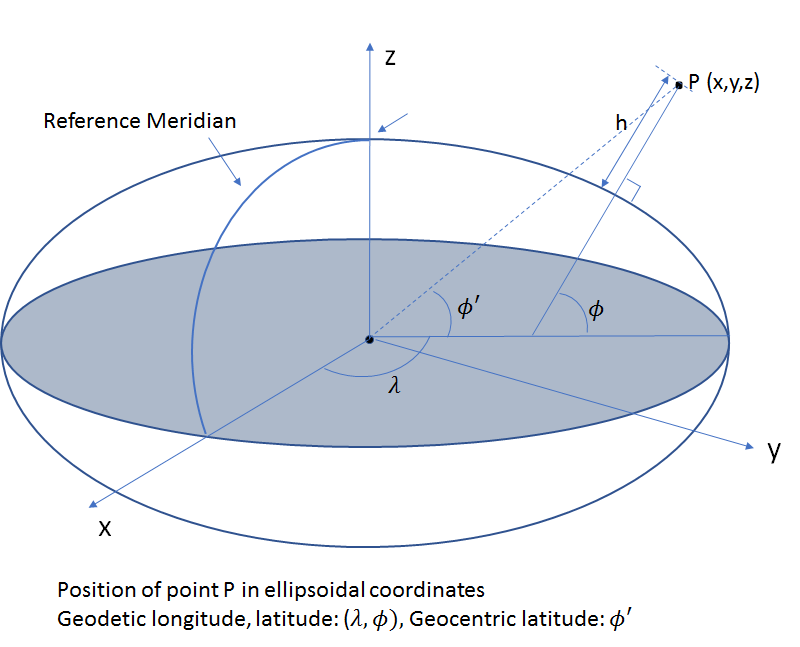
Armed with an ellipsoidal representation of the shape of the earth and with an ECEF coordinate system, we can define the position of a point P in ellipsoidal coordinates (commonly known as latitude, longitude and height) as follows:
- Geodetic Latitude (
 ): angle measured in the meridian plane through the point P between the equatorial plane of the ellipsoid and the line perpendicular to the surface of the ellipsoid at P (positive north from the equator, negative south)
 - Geodetic Longitude (
 ): angle measured in the equitorial plane between the reference meridian and the meridian plane through P (positive east from the zero meridian)
 - Geodetic height (
 ): measured along the normal to the ellipsoid through P.
Note that the latitude is the angle between the equatorial plane and the line perpendicular to the surface of the ellipse at point P, not the line joining point P and the earth center (origin of the ECEF frame). Angle between the equatorial plane and the line joining point P and the earth center is called the geocentric (as opposed to geodetic) latitude. If the earth were a perfect sphere, the normal to a point would pass through the earth center and the geocentric and geodetic latitude would coincide.
Conversion between Geodetic (Ellipsoidal) and Cartesion Coordinates
Conversion from ellipsoidal to cartesian coordinates is straightforward and can be implemented in one step.

Going from cartesian to ellipsoidal is trickier and involves an iterative procedure that quickly converges. See Appendix 4.A of 1 for details. The corresponding Matlab code is listed in section 1.e of the appendix. The more common use case is to convert ECEF coordinates to ellipsoidal as the input and output of GPS processing algorithms are usually in ECEF coordinates.
Local Coordinate Systems
So far, we have mostly talked about “global” coordinate systems, centered at the earth center. In some applications, it is more convenient to use local coordinate systems, centered on the user’s position. These coordinate systems are called East-North-Up (ENU) systems. Given the user’s position in elliptical coordinates (: latitude, : longitude), user coordinates can be easily converted from a ECEF frame to a local ENU frame using the following matrix multiplication.

We’ll see an application of ECEF to ENU conversion when we compute the azimuth and elevation of one of the GPS satellites later.
Part 2: Using GPS to Calculate User Position
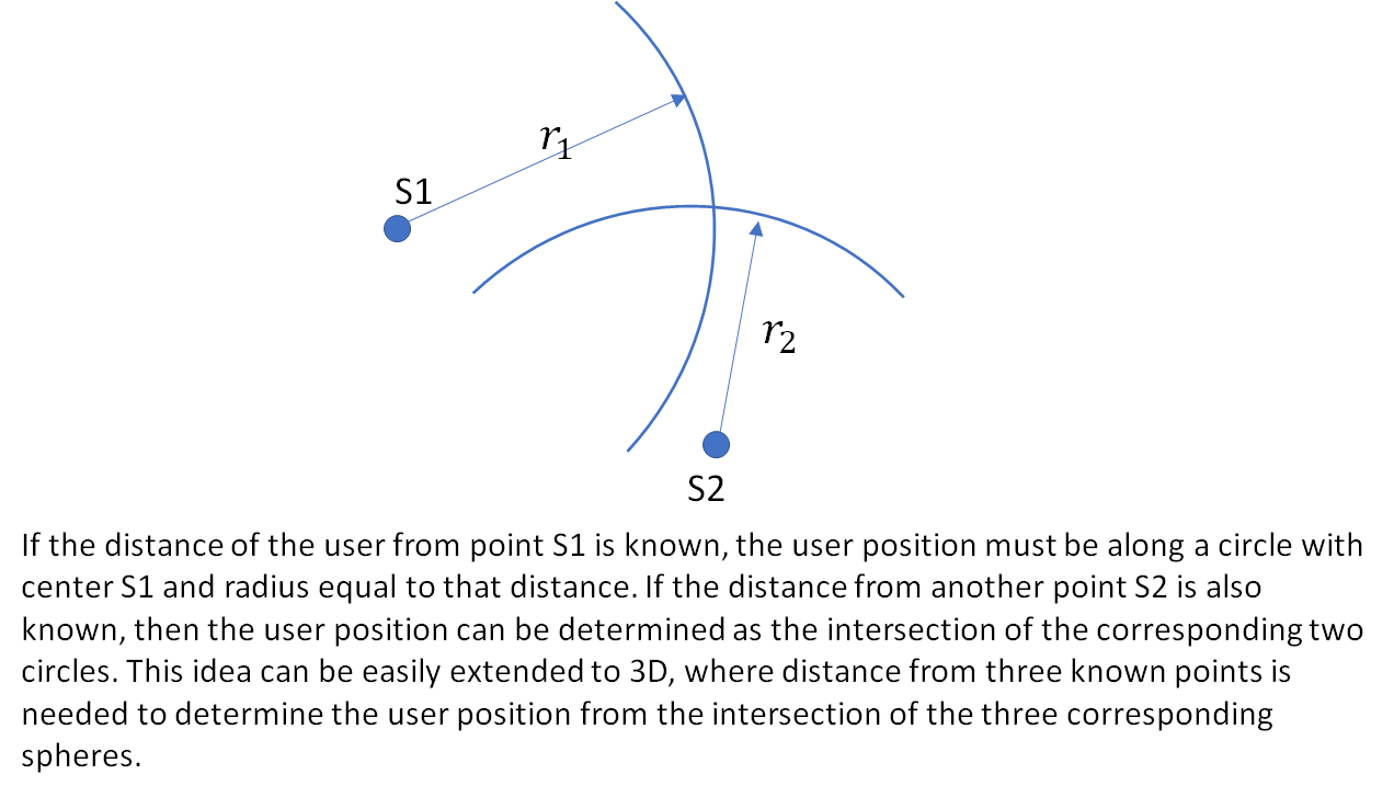
Determining the position of a user using GPS is essentially a triangulation problem. If the distance of the user from three or more satellites is known, then the 3D position can be calculated using triangulation. The basic idea in 2 dimensions is shown below.
The problem of locating the user can thus can be divided into two subproblems:
- Finding the distance of the user from each satellite
- Determining the position of this satellite in the user’s coordinate system
Let’s look at each of these problems step by step.
Step 1: Determining the Position of a Satellite
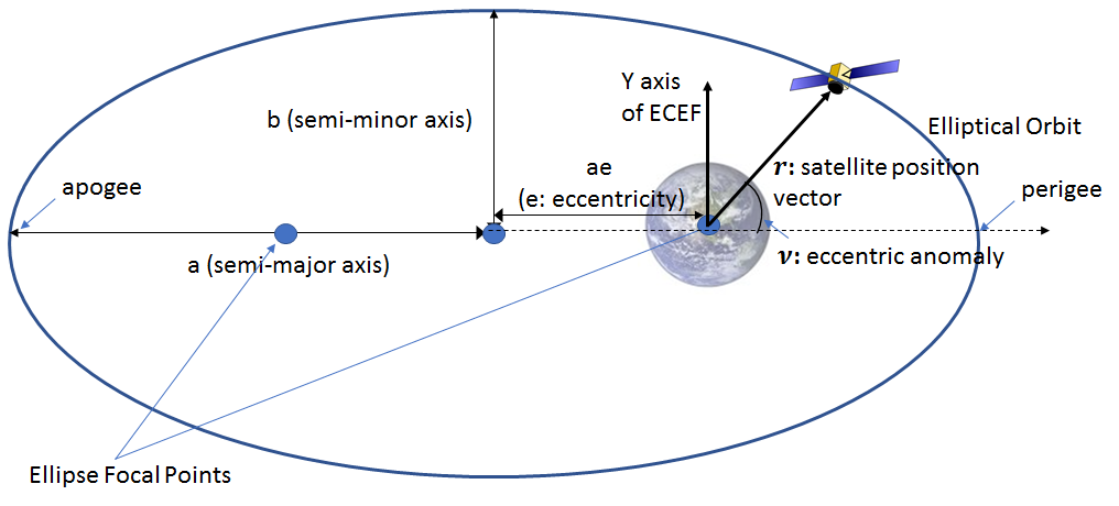
The ideal satellite orbit is an elliptical orbit and specified completely by 5 Keplerian parameters five of which determine the size and shape of the ellipse and the orientation of the orbital plane relative to the fixed stars (i.e., an inertial reference frame). The sixth parameter specifies the position of the satellite at a particular time instant of epoch. Given the six elements, the satellite position and velocity can be computed at any other epoch.
The orbit of a satellite is not an exact ellipse however as the earth is not uniform in composition and the movement of a satellite is perturbed by the gravitational forces of the sun and the moon. The resulting perturbations are small, but must be accounted for to obtain accurate position. GPS accounts for these perturbations by transmitting an expanded set of 16 orbital parameters that can be used to accurately compute the position of a satellite at a given time instant. We won’t go into the details of how these corrections are applied. The step-by-step procedure to compute the satellite position (including applying the orbital corrections) is described in table 20-IV in the GPS IS. The Matlab code that implements this procedure is shown in section 1.b of the appendix.
Rotating the Satellite Reference Frame
The user position is being calculated at time  . The GPS signal left the satellite at time
  and arrives at the user
  seconds later. While calculating the user’s position, we’ll calculate the satellite positions at , the time of signal transmission. In time interval however, the earth has rotated by
  where
where  is the rotation rate of the earth. We must rotate the satellite position vectors by the same amount, so that they are expressed in the user’s reference frame, i.e., ECEF frame at time . This is done by multiplying the satellite position vector
  by the following rotation matrix:

Note that this is not equivalent to calculating the position of the satellites at time !
Step 2: Computing the Distance of the User from the Satellite
The satellite signal received by a GPS receiver bears the time stamp at which the signal was sent from the satellite. By taking the difference between its own time and the timestamp of the GPS signal and multiplying by the speed of light, the receiver calculates a rough measure of the distance between the receiver and the satellite. This measure is called the pseudorange. If the clock on the satellite and the receiver were perfectly in sync and the GPS signal traveled in a straight line at the speed of light, then this measure would be the true distance between the satellite and the receiver. This however is not the case and the difference between the satellite and user clocks as well as the delays caused by the atmosphere must be modeled to calculate an accurate position of the user.
Let’s consider first the effect of the offset between the user and satellite clocks. Let’s denote the transmission time from the satellite to the user by and a common time reference (referred to as GPS Time (GPST)) by . Denoting the receiver clock bias at time by  and satellite clock bias at time by
  , the pseudorange
  measured by the GPS receiver is given as:
(1) ![\begin{equation*} \rho(t) = c[t+\delta{t}_u(t)-(t-\tau+\delta{t}_s(t))] + \epsilon_\rho(t) = c\tau + c[\delta{t}_u(t)-\delta{t}_s(t)] + \epsilon_\rho(t) \end{equation*}](https://telesens.co/wp-content/ql-cache/quicklatex.com-2d2d2486b0bccdeffbb6eb1a72cb10c0_l3.png "Rendered by QuickLaTeX.com")
If there wasn’t a layer of atmosphere between the satellite and the user, the satellite signal would travel along a straight line with the speed of light. Thus, the distance to the satellite at time denoted by  would be equal to
  .
.
In reality (thankfully), there is thick layer of atmosphere in the path of the satellite signal which slows it down and bends its path. The change in the path length due to bending of the signal ray is generally not significant. However the change in the speed of propagation can be significant and can result in positioning errors of several meters or more. This change in speed has two components –  arising from the propagation of the signal through the ionosphere and
  arising from the propagation of the signal through the troposphere (see appendix for more information about these delays and how they can be estimated). Thus,

Combining the above two equations and dropping the reference to measurement epoch ,
(2) ![\begin{equation*} \rho(t) = r(t, t-\tau) + I_\rho + I_\rho + c[\delta{t}_u(t)-\delta{t}_s(t)] + \epsilon_\rho(t) \end{equation*}](https://telesens.co/wp-content/ql-cache/quicklatex.com-a30ad2de80f48c4bab8ea88a66b54f60_l3.png "Rendered by QuickLaTeX.com")
Thus, the true range (actual distance of the user from a satellite) can be calculated from the raw pseudo ranges output by the GPS device by first subtracting the user’s estimate of the Tropo and Iono delays and then adjusting for the satellite clock offset. The Iono and the Tropo delay generally lead to a position error of ~25m and ~2m respectively. More information about how to estimate these delays are provided in the appendix. In the rest of our analysis in this blog, we’ll ignore these delays.
Estimating the Satellite Clock Bias
The satellite clock bias is important to estimate as it can result in a position error of thousands of meters. The procedure to calculate the satellite clock bias is described on page 96 of the GPS Interface Specification document. The procedure consists of evaluating a polynomial whose coefficients are provided in the GPS ephemeris message and adding a relativistic term. The polynomial provides most of the correction, with the relativistic effect contributing about 1-10 m depending on the position of the satellite. The code for calculating the satellite clock bias is given in section 1.d of the appendix.
User Clock Bias
The user clock bias is an unknown quantity, just like the user position. The user clock bias will be estimated along with the user position.
Step 3: User Position and Clock Bias Estimation
We are now ready to look at the algorithm used to compute the user position. A quick point about the notation before we look at the math. Generally, vector quantities are expressed using boldface ( ) and scalar quantities without emphasis. However in the math shown below, (mostly due to laziness), I’m skipping making this distinction. I think it is clear from the context which quantities are vectors and which ones are not.
Once the satellite clock bias has been accounted for and all available corrections have been applied, the corrected pseudorange measurement for satellite  can be written as
(3) 
Here  is the true distance between the user and the satellite and
  denotes the combined effect of the unmodeled errors. Note that all elements in this equation are distances. We have converted the receiver clock bias
  into a distance by multiplying by the speed of light
  . Also note that all of these calculations are carried out at time and all position vectors are expressed in the ECEF frame at time . We drop explicit reference to time for convenience.
Let the position of the user in the ECEF frame be denoted by  , and the position of satellite by
  . Then,

and

We use  to represent the user clock bias in units of distance
We wish to determine and that minimize the difference between the measured and the estimated pseudorange for each satellite. In other words, our task is to determine and such that
(4) 
is minimized for all satellites .
This problem is solved using an iterative procedure by starting with an estimate of and and finding the corrections that minimize the equation above. Let our initial estimates be denoted by  and
and  . We wish to find
  and
and  such that the true user position
  and the true clock bias
  minimize
(5) 
Here  is the unit vector from the user to satellite and we used the Taylor series expansion of the vector norm (see appendix) to express the delta pseudorange as a matrix multiplication between known and unknown quantities. Concatenating the linear equation developed above for
  satellites,

Setting

The expression above can be written more compactly as

For a non-degenerate ( are non-coplanar) configuration of =4 satellites, the equation above can be solved directly. In general, if the sky is not obstructed, many more satellites are visible, and a exact solution is not available. We can use linear algebra techniques to find a least squares solution:

The hat above the estimated quantities indicates that they are a least squares solution, not an exact solution.
The complete procedure to calculate the user position and clock bias is as follows.
|
1 2 3 4 5 6 7 8 9 10 11 12 13 14 15 16 17 18 19 20 21 22 23 24 25 26 27 28 29 30 |
Input: Raw pseudoranges, satellite ephemeris information Output: User position in ECEF and user clock bias Initialize user clock bias = 0, user position = [0 0 0] (amazing that this works!) For each satellite: 1. Calculate satellite clock bias 2. Correct measured pseudorange by the calculated satellite clock bias 3. Apply ionospheric and tropospheric corrections if available End For Do until change in user clock bias, user position < threshold For each satellite: 1. Correct pseudorange by current estimate of the user clock bias 2. Calculate signal transmission time tau by dividing pseudorange by speed of light 3. Calculate satellite position at t-tau 4. Rotate satellite position by earth's rotation in time tau to align with user's ECEF frame at time t 5. Form G matrix by concatenating unit vectors from the user to the satellite 6. Calculate delta pseudoranges by taking the difference between the corrected pesudorange (step 1) and expected pseudorange, given the current estimate of the user's position and user clock bias End For Solve for corrections in user position and clock bias and calculate new user position and clock bias End Do |
Note about the Matlab Code
It is worth noting that while most of the equations in the Matlab code shown in the Appendix involve evaluation of expressions where the known quantities are on the right hand side and unknown quantities on the left hand side (and thus can be evaluated in one step), there are a few that requires invocation of a solver. One example is the calculation of the eccentric anomaly (E) from the mean anomaly (M) required during the calculation of the satellite position from ephemeris parameters. The relation between the two is expressed as:

where  is the eccentricity of the earth’s orbit. Typically,
  is calculated first, and calculating
  from can’t be done in closed form and requires the use of a solver. Part of the code is shown below.
|
1 2 3 4 5 6 |
% mk: Mean anomaly % solve for eccentric anomaly syms E; eqn = E - eph.e*sin(E) == mk; solx = vpasolve(eqn, E); Ek = double(solx); |
Experimental Setup
In this section, I’ll describe the hardware setup I used to collect raw GPS data which was then processed using the algorithms described above to calculate user position and clock bias. An interested user should be able to easily replicate my setup using cheap and commercially available GPS receivers and open source software.
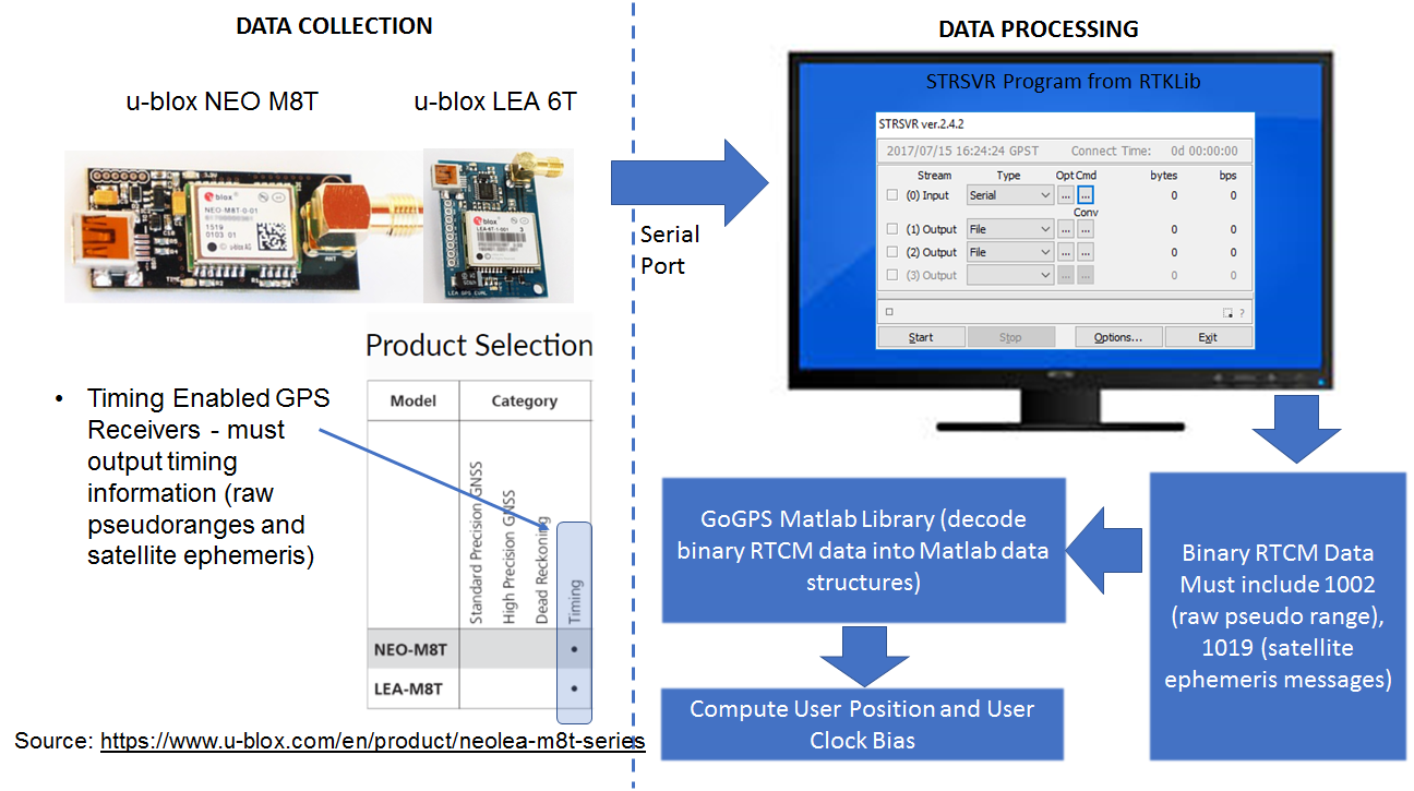
The figure above shows the main steps involved in my setup. For collecting raw GPS data, special GPS units that output “timing” information consisting of raw pseudoranges and satellite ephemeris information must be used. Regular GPS units calculate the user position internally and don’t output the raw data we need to calculate the user position using the algorithm described above. The NEO-M8T and 6T chips from u-blox fit our needs. Complete hardware assemblies with the GPS unit, antennae and serial output port can be purchased from Amazon for ~40 dollars.
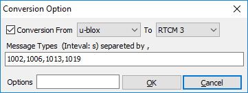
In order to receive and save the raw GPS signal, I use the STRSVR utility in RTKLib (RTKLIB is an open source program package for standard and precise positioning that supports all common Global Navigation Satellite Systems (GNSS) – GPS, Glonass, Galileo, Baidu etc. See: http://www.rtklib.com). STRSVR takes the custom u-blox formatted output from the u-blox receiver and converts it into RTCM standard format. RTCM (Radio Technical Commission for Maritime Services, see: http://www.rtcm.org/differential-global-navigation-satellite–dgnss–standards.html) is a standard for GNSS data and content designed to support a variety of GNSS applications in air/land/sea navigation, surveying, radio navigation/location etc.
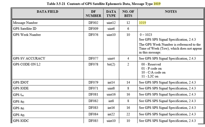
RTCM standard provides the definition of various messages that provide specific GPS information. The information we are interested in are the raw pseudoranges and satellite ephemeris. This information is contained in messages 1002 and 1019.
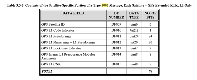
We must request the u-blox receiver to send 1002 and 1019 message information as part of the data it sends to STRSVR. This is done by using the following commands in the Cmd window:
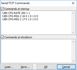
The first command sets the update rate to 1Hz and the other two enable RAW messages. The details on how this happens are a bit murky. I tried going through parts of the UBX documentation to understand this better but soon got lost. Suffices to say that the above commands work and cause the receiver to send the data we need.
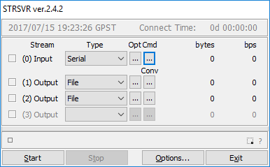
I configure the STRSVR utility to receive data from the serial port at 9600 Baud and save the data to a file in RTCM 3 format.
To collect the data, I went to the roof of my apartment building and placed the GPS receiver at a location where it could get an unobstructed view of the sky. I used the u-blox configuration software (https://www.u-blox.com/en/product/u-center-windows) to verify that a sufficient number of satellites were visible and a good position fix could be obtained. I then used STRSVR to collect about an hour of raw GPS data and saved the data to a file.
Processing Raw GPS Data
STRSVR saves the raw GPS data into binary RTCM3 format. We must decode the RTCM3 data to create Matlab data structures out of it. I considered writing my own RTCM decoder, but then found an excellent Matlab library called goGPS (http://www.gogps-project.org/about/) that provides many useful routines to read and process GPS data. I used the load_stream function that reads an RTCM formatted file and extracts the RTCM messages (line 95 in my version of goGPS). I then saved the extracted data to a .mat file to serve as input to my the position calculation algorithm that implements the equations above. The Matlab code is shown in the section 1.a of the appendix. I’m also attaching the rtcm_data since many people have asked for it. I changed the file extension from .mat to .txt due to wordpress security restrictions. Rename the file back to .mat when you download it.
Analysis of Results
In this section, I’ll analyze the positions and clock bias computed by my algorithms. We will look at the variation of the north/east/up components of the position with time, variation of the clock bias with time and introduce the concept of Dilution of Precision (DOP), a common metric used to measure the quality of GPS position estimates. Since the GPS receiver was stationary during data collection, the variation of the calculated position reflects the true performance of the algorithm used to calculate the position.
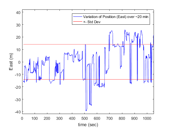
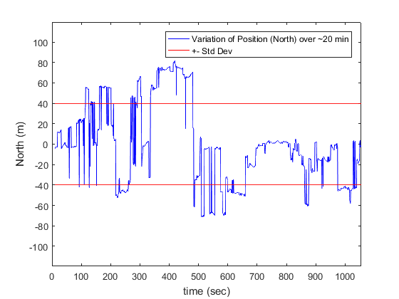
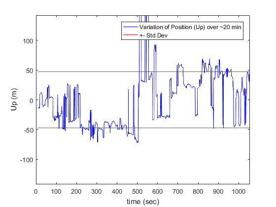
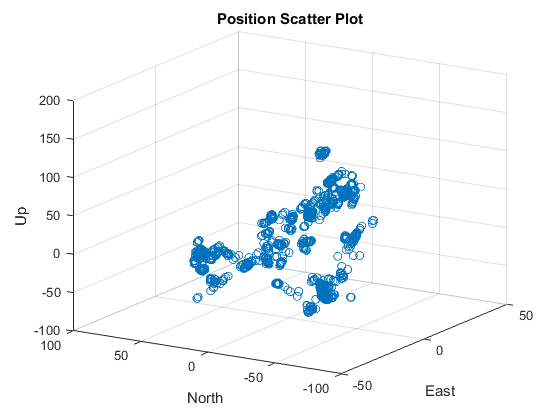
| East | North | Up | |
| Std-Dev | 14.00 | 39.88 | 47.35 |
The plot of E/N/U components of the user position in a user centered ENU frame along with the position scatter plot are shown above. As expected, the variation in position is around 30m in the East and North direction and slightly higher along the Up direction. We’ll explain the reason for this during the discussion about DOP (Dilution of Precision) below.
Clock Bias Drift
The variation of the receiver clock bias against time is shown below. Note that the clock bias used in the algorithm above is in the unit of distance. In the plot below, the bias has been converted into unit of time by dividing by the speed of light.
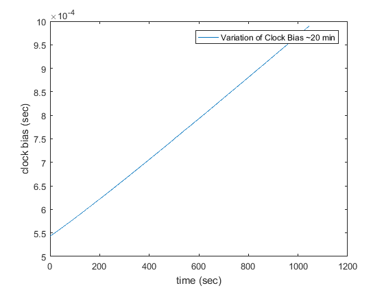
We can see that the clock bias is not a constant but drifts linearly with time. The amount of drift is 4.27 e-7sec/sec.
Computing the Satellite Azimuth/Elevation
As an exercise, let’s compute the azimuth and elevation of all the satellites visible at a given time instant. This will neatly tie in many of the ideas discussed above and also provide a good segue to discussing DOP.
Azimuth and elevation angles are calculated from the perspective of the user. Thus, they are expressed in an ENU frame centered about the user position.
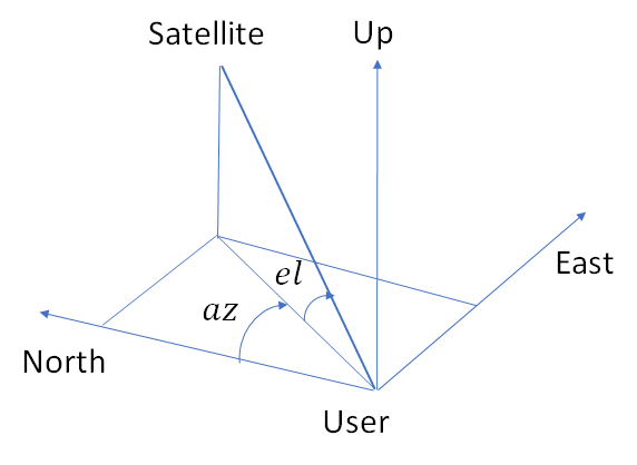
If the position of the satellite in the user centered ENU frame is ( ), then the azimuth (az) and elevation (el) is given by:


The procedure to extract azimuth and elevation from satellite and user positions (calculated in the ECEF frame) is as follows:
- Calculate the position vector from the user to the satellite (in ECEF frame)
- Calculate the user position in Ellipsoidal coordinates (lat/lng)
- Rotate the position vector to the ENU frame centered about the user position
- Calculate azimuth/elevation using equations above)
The Matlab code is shown below:
|
1 2 3 4 5 6 7 8 9 10 11 12 13 14 15 16 |
function [az el] = get_satellite_az_el(xs,ys,zs,xu,yu,zu) % get_satellite_az_el: computes the satellite azimuth and elevation given % the position of the user and the satellite in ECEF % Usage: [az el] = get_satellite_az_el(xs,ys,zs,xu,yu,zu) % Input Args: xs,ys,zs: satellite position in ECEF % xu,yu,zu: user position in ECEF % Output Args: azimuth and elevation [lambda, phi, h] = WGStoEllipsoid(xu,yu,zu); lat = phi*180/pi; lng = lambda*180/pi; enu =Rotxyz2enu([xs-xu,ys-yu,zs-zu]', lat, lng); az = atan2(enu(1), enu(2)); el = asin(enu(3)/norm(enu)); % The azimuth and elevation end |
The computed azimuth and elevations at a given epoch are shown in the table and the corresponding 3D positions in the ENU frame are shown in the plot below
| Azimuth | Elevation |
| 69.68 | 62.89 |
| -20.46 | 81.63 |
| 96.38 | 16.91 |
| 34.71 | 5.21 |
| -145.06 | 12.59 |
| -165.22 | 7.44 |
| -110.29 | 39.03 |
| -49.30 | 43.11 |
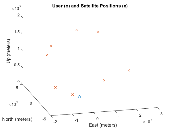
As can be seen the azimuth angles are both positive and negative, while the elevations are only positive. This makes sense as the user can’t see the satellites below the horizon.
You may have seen satellite track charts that many GPS processing software output as a visualization aid. Those charts are created by calculating the satellite positions using the procedure described here at multiple epochs.
Dilution of Precision (DOP)
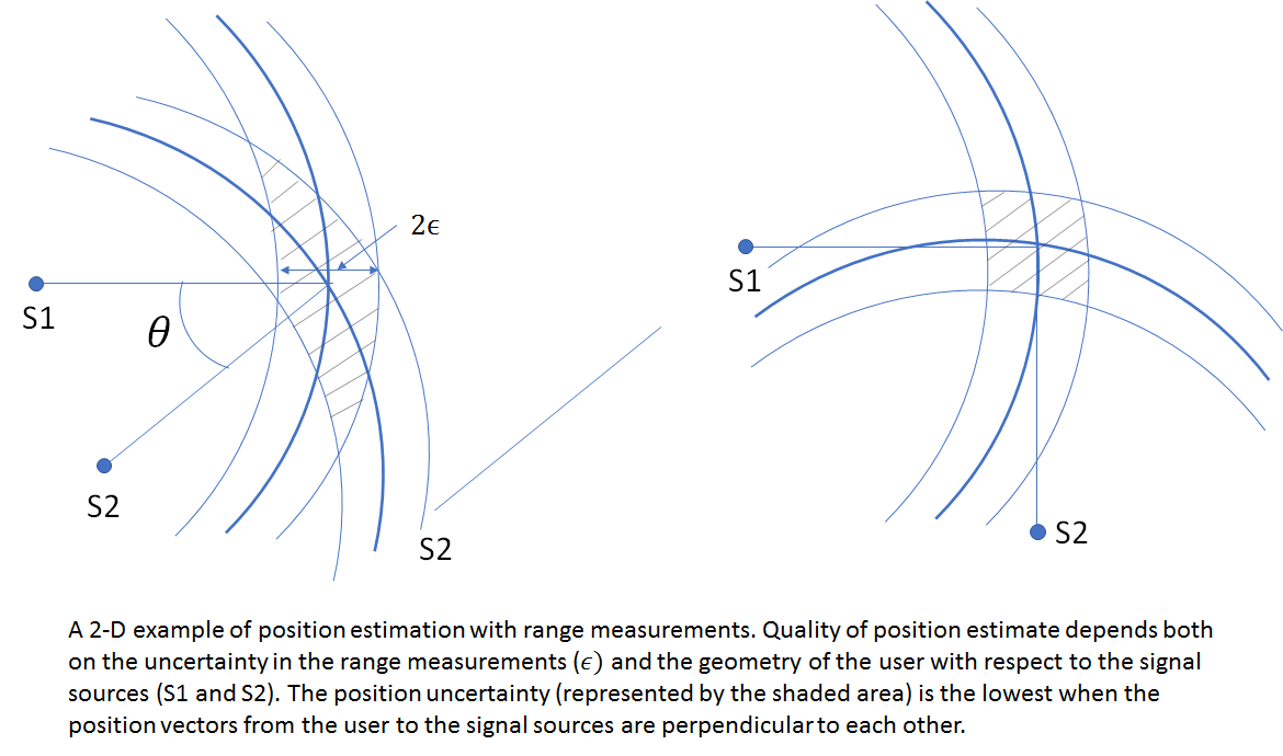
DOP helps us answer the question, “how good are my position estimates”? There are two components of the errors in our position estimate. The first one is the measurement noise, which is obvious. The noisier our measurements (pseudorange, satellite position etc), higher are the expected position errors. However, there is another, less obvious component of the positioning errors. This component is the user-satellite geometry. As explained in chapter 6 of 1, it the easiest to see this in a 2D example.
A user measures his distance from a pair of signal sources S1 and S2 at known locations. If the range measurements were perfect, the user could determine his position exactly as lying on the intersection of two circles centered on S1 and S2 and radii equal to the measured ranges. The measurements however are imperfect and have a maximum uncertainty of  . The figure below shows how the user-source geometry affects the amount of uncertainty in the user position.
The uncertainty in the position and clock bias is measured by the covariance of the estimated position and clock bias error. Representing the true position and clock bias by and , the position and clock bias estimation errors are given as:


Where  and
and  are our estimates of the user position and clock bias (calculated using the algorithm above). As shown in chapter 6 of 1, the covariance matrix of position and clock bias is given as:

Here  is the “user range error” which captures the uncertainty in the pseudoranges and satellite positions. The
  matrix is the matrix consisting of the unit vectors from the user to the satellite that we saw earlier. This matrix depends entirely on the user-satellite geometry. Thus, the covariance can be neatly factored into a product of measurement uncertainty and a function of the user-satellite geometry matrix. The elements of the G matrix are expressed in the ECEF frame. It is more convenient to rotate it into the user’s local ENU frame. Let
  be the required rotation matrix and
  be the resulting geometry matrix.
![\tilde{G} = [G(1:N, 1:3)R_L^{T}, ones(N,1)]](https://telesens.co/wp-content/ql-cache/quicklatex.com-7c1784d95cd84a75737e6cd27eeaf054_l3.png "Rendered by QuickLaTeX.com")
Here  is the number of satellites. The rotation is applied to the position components of the geometry matrix. it can be easily shown that

Setting
 ,
,
The East, North and Up components of DOP are defined as

We can further define a horizontal DOP (HDOP) by combining the E and N term (since the East and North directions define the horizontal plane at the user’s location) and vertical DOP (VDOP) consisting of the U term.


DOP provides a simple characterization of the user-satellite geometry. The more favourable the geometry, the lower the DOP. More favourable means the satellites are spread apart in azimuth and elevation. The lower the DOP and user range error (), the better the quality of the position estimate. To understand the relationship between DOP and satellite geometry better, lets consider two simple examples. The first example looks at the variation between DOP and the angle between the satellite vectors in a three satellite configuration shown in the figure below. The first satellite is located along the y axis and the other two are located symmetrically about the y axis, at an angle  from the x-axis. The G matrix and the plot of DOP against angle theta is shown below.
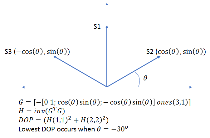
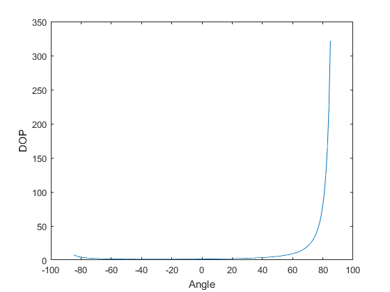
The minimum DOP occurs at  . This makes intuitive sense as at this angle, the satellites are maximally separated from each other. Note that the DOP does not vary symmetrically with positive and negative . This is because for a given , the separation between the satellite vectors is higher for a negative value than for a positive value.
Next let’s look at a more realistic example of four satellites located in 3D. First satellite is located at the zenith and the others three are located 120 degrees apart in azimuth and at an elevation of (same for the three satellites). We’ll look at the variation of VDOP with the elevation angle.
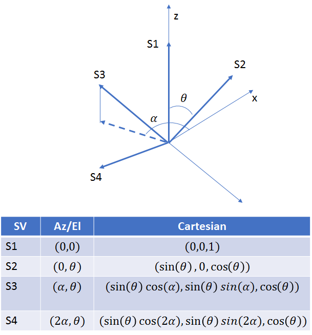
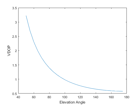
As expected, the VDOP decreases with increasing elevation angle, as the satellites get farther apart from each other. It continues to decrease as the elevation goes past the horizon (elevation = 90 degrees). Since a user located on the earth surface can’t observe satellites below the horizon (in fact, signal from satellites < 10 degrees above the horizon are too noisy and generally not used), the minimum value of VDOP is not achievable. This example demonstrates why VDOP is generally higher than HDOP.
Let’s now look at the variation of HDOP and VDOP with time calculated by our position algorithm on real data.
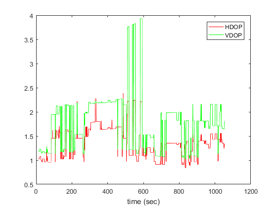
No surprises here. The HDOP/VDOP values are generally < 2.5, which is considered adequate and as expected, VDOP is higher than HDOP.
This concludes the post! I hope that next time you use Google maps to get directions, you’ll think about the incredible scientists, engineers and policy makers who have given us this incredible system that makes possible so many applications that we now take for granted. According to 1, the GPS constellation cost about 30 billion dollars to put in place and costs the US government about 1B annually to maintain. The valuation of Uber alone, which wouldn’t exist without GPS is upwards of 70B dollars. When you include all of the other amazing applications made possible by GPS, the public investment in GPS appears to be one of the best public investments ever made! 🙂
Appendix
1.a Code for Calculating User Position and Clock Bias
|
1 2 3 4 5 6 7 8 9 10 11 12 13 14 15 16 17 18 19 20 21 22 23 24 25 26 27 28 29 30 31 32 33 34 35 36 37 38 39 40 41 42 43 44 45 46 47 48 49 50 51 52 53 54 55 56 57 58 59 60 61 62 63 64 65 66 67 68 69 70 71 72 73 74 75 76 77 78 79 80 81 82 83 84 85 86 87 88 89 90 91 92 93 94 95 96 97 98 99 100 101 102 103 104 105 106 107 108 109 110 111 112 113 114 115 116 117 118 119 120 121 122 123 124 125 126 127 128 129 130 131 132 133 134 135 136 137 138 139 140 141 142 143 144 145 146 147 148 149 150 151 152 153 154 155 156 157 158 159 160 161 162 163 164 165 166 167 168 169 170 171 172 173 174 175 176 177 178 179 180 181 182 183 184 185 186 187 188 189 190 191 192 193 |
% Constants that we will need % Speed of light c = 299792458; % Earth's rotation rate omega_e = 7.2921151467e-5; %(rad/sec) % load out data data = load('rtcm_data.mat'); % Data is a cell array containing data about different RTCM messages. We % are interested in 1002 and 1019 % msgs is a an array of message ids (1002, 1019 etc) msgs = [data.data{1,:}]; % Get indicies of ephemeris info (msg 1019) [idx_1019] = find(msgs == 1019); % Get indicies of raw pseudorange info (msg 1002) [idx_1002] = find(msgs == 1002); % Satellite ephemeris data is all mixed up since different satellites are visible at % different epocks. eph = [data.data{2, idx_1019}]; % Lets group data for each satellite % find unique satellite indicies sv_arr = unique(eph(1,:)); % eph_data will contain ephemeris data for all epochs grouped by satellite % number eph_data = {}; for i = 1: length(sv_arr) % find indicies of all entries corresponding to this satellite sv = sv_arr(i); idx = find(eph(1,:) == sv); eph_data{sv} = eph(:,idx); end % Now let's deal with 1002 messages. 1002 messages have two entries - first % one (nav1) is a 6*1 array containing: reference station id, receiver time % of week, number of satellites etc. See decode_1002.m in goGPS for details % The important pieces of info in nav1 are the receiver time of week and the % number of satellites visible % The second one (nav2) contains a block of 56*5 for every epoch. % Num of rows (56) refers to the maximum number of satellites in the % constellation. Num of cols (5) is the number of data elements for each satellite. % We are interested in the second element, the raw pseudorange. % For those satellites for which no info is available, % the rows of nav2 contain 0s. nav1 = [data.data{2, idx_1002}]; nav2 = [data.data{3, idx_1002}]; len = length(nav1); % Arrays to store various outputs of the position estimation algorithm user_position_arr = []; HDOP_arr = []; VDOP_arr = []; user_clock_bias_arr = []; % initial position of the user xu = [0 0 0]; % initial clock bias b = 0; % 1002 messages are spaced apart 200ms. Let's use 1 out of every 5 samples. % This means that we'll compute position every second, which is sufficient for idx = 1: 5: len % second element of nav1 contains receiver time of week rcvr_tow = nav1(2,idx); % data block corresponding to this satellite nav_data = nav2(:, 5*(idx-1)+1: 5*idx); % find indicies of rows containing non-zero data. Each row corresponds % to a satellite ind = find(sum(nav_data,2) ~= 0); numSV = length(ind); eph_formatted_ = []; % The minimum number of satellites needed is 4, let's go for more than % that to be more robust if (numSV > 4) pr_ = []; % Correct for satellite clock bias and find the best ephemeris data % for each satellite. Note that satellite ephemeris data (1019) is sent % far less frequently than pseudorange info (1002). So for every % epoch, we find the closest (in time) ephemeris data. for i = 1: numSV, sv_idx = ind(i); sv_data = nav_data(sv_idx,:); % find ephemeris data closest to this time of week [c_ eph_idx] = min(abs(eph_data{sv_idx}(18,:)-rcvr_tow)); eph_ = eph_data{sv_idx}(:, eph_idx); % Convert the ephemeris data into a standard format so it can % be input to routines that process it to calculate satellite % position and satellite clock bias eph_formatted = format_ephemeris3(eph_); eph_formatted_{end+1} = eph_formatted; % To be correct, the satellite clock bias should be calculated % at rcvr_tow - tau, however it doesn't make much difference to % do it at rcvr_tow dsv = estimate_satellite_clock_bias(rcvr_tow, eph_formatted); % measured pseudoranges corrected for satellite clock bias. % Also apply ionospheric and tropospheric corrections if % available pr_raw = sv_data(2); pr_(end+1) = pr_raw + c*dsv; end % Now lets calculate the satellite positions and construct the G % matrix. Then we'll run the least squares optimization to % calculate corrected user position and clock bias. We'll iterate % until change in user position and clock bias is less than a % threhold. In practice, the optimization converges very quickly, % usually in 2-3 iterations even when the starting point for the % user position and clock bias is far away from the true values. dx = 100*ones(1,3); db = 100; while(norm(dx) > 0.1 && norm(db) > 1) Xs = []; % concatenated satellite positions pr = []; % pseudoranges corrected for user clock bias for i = 1: numSV, % correct for our estimate of user clock bias. Note that % the clock bias is in units of distance cpr = pr_(i) - b; pr = [pr; cpr]; % Signal transmission time tau = cpr/c; % Get satellite position [xs_ ys_ zs_] = get_satellite_position(eph_formatted_{i}, rcvr_tow-tau, 1); % express satellite position in ECEF frame at time t theta = omega_e*tau; xs_vec = [cos(theta) sin(theta) 0; -sin(theta) cos(theta) 0; 0 0 1]*[xs_; ys_; zs_]; xs_vec = [xs_ ys_ zs_]'; Xs = [Xs; xs_vec']; end % Run least squares to calculate new user position and bias [x_, b_, norm_dp, G] = estimate_position(Xs, pr, numSV, xu, b, 3); % Change in the position and bias to determine when to quite % the iteration dx = x_ - xu; db = b_ - b; xu = x_; b = b_; end % end of iteration % Convert from ECEF to lat/lng [lambda, phi, h] = WGStoEllipsoid(xu(1), xu(2), xu(3)); % Calculate Rotation Matrix to Convert ECEF to local ENU reference % frame lat = phi*180/pi lon = lambda*180/pi R1=rot(90+lon, 3); R2=rot(90-lat, 1); R=R2*R1; G_ = [G(:,1:3)*R' G(:,4)]; H = inv(G_'*G_); HDOP = sqrt(H(1,1) + H(2,2)); VDOP = sqrt(H(3,3)); % Record various quantities for saving and plotting HDOP_arr(end+1,:) = HDOP; VDOP_arr(end+1,:) = VDOP; user_position_arr(end+1,:) = [lat lon h]; user_clock_bias_arr(end+1,:) = b; end end HDOP_arr; %Function R=rot(angle (degrees), axis) returns a 3x3 %rotation matrix for rotating a vector about a single %axis. Setting axis = 1 rotates about the e1 axis, %axis = 2 rotates about the e2 axis, axis = 3 rotates %about the e3 axis. function R=rot(angle, axis) %function R=rot(angle (degrees), axis) R=eye(3); cang=cos(angle*pi/180); sang=sin(angle*pi/180); if (axis==1) R(2,2)=cang; R(3,3)=cang; R(2,3)=sang; R(3,2)=-sang; end; if (axis==2) R(1,1)=cang; R(3,3)=cang; R(1,3)=-sang; R(3,1)=sang; end; if (axis==3) R(1,1)=cang; R(2,2)=cang; R(2,1)=-sang; R(1,2)=sang; end; return; end |
1.b Code for Calculating Satellite Position
|
1 2 3 4 5 6 7 8 9 10 11 12 13 14 15 16 17 18 19 20 21 22 23 24 25 26 27 28 29 30 31 32 33 34 35 36 37 38 39 40 41 42 43 44 45 46 47 48 49 50 51 52 53 54 55 56 57 58 59 60 61 62 63 64 65 66 67 68 69 70 71 72 73 74 75 76 77 78 79 80 81 82 83 84 85 86 87 88 89 90 91 92 93 94 |
function [x y z] = get_satellite_position(eph, t, compute_harmonic_correction) % get_satellite_position: computes the position of a satellite at time (t) given the % ephemeris parameters. % Usage: [x y z] = get_satellite_position(eph, t, compute_harmonic_correction) % Input Args: eph: ephemeris data % t: time % compute_harmonic_correction (optional): 1 if harmonic % correction should be applied, 0 if not. % Output Args: [x y z] in ECEF in meters % ephmeris data must have the following fields: % rcvr_tow (receiver tow) % svid (satellite id) % toc (reference time of clock parameters) % toe (referece time of ephemeris parameters) % af0, af1, af2: clock correction coefficients % ura (user range accuracy) % e (eccentricity) % sqrtA (sqrt of semi-major axis) % dn (mean motion correction) % m0 (mean anomaly at reference time) % w (argument of perigee) % omg0 (lontitude of ascending node) % i0 (inclination angle at reference time) % odot (rate of right ascension) % idot (rate of inclination angle) % cus (argument of latitude correction, sine) % cuc (argument of latitude correction, cosine) % cis (inclination correction, sine) % cic (inclination correction, cosine) % crs (radius correction, sine) % crc (radius correction, cosine) % iod (issue of data number) % set default value for harmonic correction switch nargin case 2 compute_harmonic_correction=1; end mu = 3.986005e14; omega_dot_earth = 7.2921151467e-5; %(rad/sec) % Now follow table 20-IV A = eph.sqrtA^2; cmm = sqrt(mu/A^3); % computed mean motion tk = t - eph.toe; % account for beginning of end of week crossover if (tk > 302400) tk = tk-604800; end if (tk < -302400) tk = tk+604800; end % apply mean motion correction n = cmm + eph.dn; % Mean anomaly mk = eph.m0 + n*tk; % solve for eccentric anomaly syms E; eqn = E - eph.e*sin(E) == mk; solx = vpasolve(eqn, E); Ek = double(solx); % True anomaly: nu = atan2((sqrt(1-eph.e^2))*sin(Ek)/(1-eph.e*cos(Ek)), (cos(Ek)-eph.e)/(1-eph.e*cos(Ek))); %Ek = acos((e + cos(nu))/(1+e*cos(nu))); Phi = nu + eph.w; du = 0; dr = 0; di = 0; if (compute_harmonic_correction == 1) % compute harmonic corrections du = eph.cus*sin(2*Phi) + eph.cuc*cos(2*Phi); dr = eph.crs*sin(2*Phi) + eph.crc*cos(2*Phi); di = eph.cis*sin(2*Phi) + eph.cic*cos(2*Phi); end u = Phi + du; r = A*(1-eph.e*cos(Ek)) + dr; % inclination angle at reference time i = eph.i0 + eph.idot*tk + di; x_prime = r*cos(u); y_prime = r*sin(u); omega = eph.omg0 + (eph.odot - omega_dot_earth)*tk - omega_dot_earth*eph.toe; x = x_prime*cos(omega) - y_prime*cos(i)*sin(omega); y = x_prime*sin(omega) + y_prime*cos(i)*cos(omega); z = y_prime*sin(i); end |
1.c Code for Computing the Least Squares Solution for User Position and Clock Bias
|
1 2 3 4 5 6 7 8 9 10 11 12 13 14 15 16 17 18 19 20 21 22 23 24 25 26 27 28 29 30 31 32 33 34 35 36 37 38 39 |
function [x, b, norm_dp, G] = estimate_position(xs, pr, numSat, x0, b0, dim) % estimate_position: estimate the user's position and user clock bias % Usage: [x, b, norm_dp, G] = estimate_position(xs, pr, numSat, x0, b0, dim) % Input Args: xs: satellite position matrix % pr: corrected pseudo ranges (adjusted for known value of the % satellite clock bias) % numSat: number of satellites % x0: starting estimate of the user position % b0: starting point for the user clock bias % dim: dimensions of the satellite vector. 3 for 3D, 2 for 2D % Notes: b and b0 are usually 0 as the current estimate of the clock bias % has already been applied to the input pseudo ranges. % Output Args: x: optimized user position % b: optimized user clock bias % norm_dp: normalized pseudo-range difference % G: user satellite geometry matrix, useful for computing DOPs dx = 100*ones(1, dim); db = 0; norm_dp = 100; numIter = 0; b = b0; %while (norm_dp > 1e-4) while norm(dx) > 1e-3 norms = sqrt(sum((xs-x0).^2,2)); % delta pseudo range: dp = pr - norms + b - b0; G = [-(xs-x0)./norms ones(numSat,1)]; sol = inv(G'*G)*G'*dp; dx = sol(1:dim)'; db = sol(dim+1); norm_dp = norm(dp); numIter = numIter + 1; x0 = x0 + dx; b0 = b0 + db; end x = x0; b = b0; end |
1.d Code for Calculating Satellite Clock Bias
|
1 2 3 4 5 6 7 8 9 10 11 12 13 14 15 16 17 18 19 20 21 22 23 24 25 26 27 |
function dsv = estimate_satellite_clock_bias(t, eph) F = -4.442807633e-10; mu = 3.986005e14; A = eph.sqrtA^2; cmm = sqrt(mu/A^3); % computed mean motion tk = t - eph.toe; % account for beginning or end of week crossover if (tk > 302400) tk = tk-604800; end if (tk < -302400) tk = tk+604800; end % apply mean motion correction n = cmm + eph.dn; % Mean anomaly mk = eph.m0 + n*tk; % solve for eccentric anomaly syms E; eqn = E - eph.e*sin(E) == mk; solx = vpasolve(eqn, E); Ek = double(solx); dsv = eph.af0 + eph.af1*(t-eph.toc) + eph.af2*(t-eph.toc)^2 + F*eph.e*eph.sqrtA*sin(Ek); end |
1.e Code for converting ECEF (WGS84) to Ellipsoidal Coordinates
|
1 2 3 4 5 6 7 8 9 10 11 12 13 14 15 16 17 18 19 20 21 22 23 24 25 26 27 |
function [lambda, phi, h] = WGStoEllipsoid(x,y,z) % WGStoEllipsoid Convert ECEF coordinates to Ellipsoidal (longitude, latitude, height above ellipsoid) % Usage: [lambda, phi, h] = WGStoEllipsoid(x,y,z) % Input Args: coordinates in ECEF % Output Args: Longitude, Latitude in radians, height in meters % WGS ellipsoid params a = 6378137; f = 1/298.257; e = sqrt(2*f-f^2); % From equation 4.A.3, lambda = atan2(y,x); p = sqrt(x^2+y^2); % initial value of phi assuming h = 0; h = 0; phi = atan2(z, p*(1-e^2)); %4.A.5 N = a/(1-(e*sin(phi))^2)^0.5; delta_h = 1000000; while delta_h > 0.01 prev_h = h; phi = atan2(z, p*(1-e^2*(N/(N+h)))); %4.A.5 N = a/(1-(e*sin(phi))^2)^0.5; h = p/cos(phi)-N; delta_h = abs(h-prev_h); end end |
1.f format_ephemeris3.m
|
1 2 3 4 5 6 7 8 9 10 11 12 13 14 15 16 17 18 19 20 21 22 23 24 25 26 27 28 29 |
function eph = format_ephemeris3(eph_) eph = []; eph.svid = eph_(1); eph.toc = eph_(21); eph.toe = eph_(18); eph.af0 = eph_(19); eph.af1 = eph_(20); eph.af2 = eph_(2); eph.ura = eph_(26); % check eph.e = eph_(6); eph.sqrtA = eph_(4); eph.dn = eph_(5); eph.m0 = eph_(3); eph.w = eph_(7); eph.omg0 = eph_(16); eph.i0 = eph_(12); eph.odot = eph_(17); %eph.wdot = eph_(17); eph.idot = eph_(13); eph.cus = eph_(9); eph.cuc = eph_(8); eph.cis = eph_(15); eph.cic = eph_(14); eph.crs = eph_(11); eph.crc = eph_(10); eph.iod = eph_(22); eph.GPSWeek = eph_(24); end |
2.a Taylor Series Expansion of Vector Modulus
In the derivation of the position estimation formula, we used the taylor series expansion of the modulus function. The proof is as follows:

First two terms of the taylor series expansion of  about are:


2.b Ionospheric and Tropospheric Delay
The passage of the satellite signal through the earth’s atmosphere changes the speed of the signal and bends the signal path. These effects result in the distance to the satellite calculated by multiplying the time delay between signal transmission and reception with the speed of light to be different from the true distance. Estimating the effect of the atmosphere is important to calculate accurate pseudoranges and thus accurate user position. In the treatment above, we neglected the atmospheric effects. In this section, we’ll provide some information about atmospheric effects and how they are typically modeled. The interested reader is referred to chapter 5 of 1 for details.
For the purpose of analyzing its interaction with GPS signals, the earth’s atmosphere can be split into two parts – troposphere and the ionosphere. The ionosphere extends from a height of about 50km to about 1000km above the earth is a region of ionized gases. The ionization is caused by the sun’s radiation and the state of the ionosphere is determined primarily by the intensity of solar activity. Electron density generally builds up during the day as the sun rises, peaking at around 2 PM local time and then starts declining. There can be considerable variability from day to day depending upon the solar activity. The speed of propagation of the signal in the ionosphere depends upon the number of free electrons in the path of the signal, defined as the total electron count (TEC). The number of electrons in a tube of 1 cross section extending from the receiver to the satellite is given as:

where  is the electron density along the signal path and the integral is along the signal path from the satellite to the receiver. The path length through the ionospheric is shortest in the zenith direction (when the satellite is directly overhead) and longest when the satellite is close to the horizon.
In general, ionosphere delays are hard to model as solar flares and magnetic storms can large and rapidly varying fluctuations in electron densities. Two methods are primarily used to estimate ionospheric delays. The first method uses dual frequency GPS measurements and the fact that the ionospheric delay is inversely proportional to the square of the frequency. This enables us to set up a system of equations to estimate the ionosphere free pseudoranges from the noisy pseudoranges.
Receivers limited to single frequency measurements can use an empirical model called the Klobuchar model parameterized by the user’s latitude, longitude, satellite azimuth/elevation, local time and a set of parameters broadcast by the satellites. A step by step implementation of this model is detailed in the GPS Interface Specification and can be easily implemented in Matlab or C.
The troposphere extends to about 16 Km above the equator and contains roughly three quarters of the gaseous mass of the atmosphere. The troposphere is primarily composed of the dry gasses – nitrogen and oxygen, and water vapour. The primary effect of the troposphere on GPS signal propagation is to delay it slightly, causing the apparent range to the satellite to appear longer by about 2.5m, depending on the satellite elevation angle. Unlike the ionosphere, the troposphere is non-dispersive for GPS frequencies, and thus the tropospheric effect can’t be estimated by dual frequency measurements. The amount of delay caused by the troposphere depends on the pressure, temperature and humidity. Various models exist to calculate the delay from meteorological measurements. Refer to chapter 5 of 1 for details.
2.c Plotting code
Some people have asked for the plotting code – here it is.
can anyone suggest matlab code to plot receiver position of the satellite
I’ll send you the plotting code in a couple of days.
Hi sir,
can you suggest the python code?
It would be helpful if you provide the code.
Also please suggest Matlab code to plot receiver position of the satellite
Thank you
I’m unable to support requests such as these. I’m not actively working on GPS anymore, and can’t provide support for custom code requests. The Matlab code provided with this post is complete and people have been able to use the Matlab code provided to recreate the results shown. Please refer to Matlab documentation and stackoverflow for custom code requests.
Hi ankur,
you did a really good work here!
Thanks for sharing this with us.
Using your code I was able to recreate your results you have shown here.
So for every other user I can say that this code works as it should be.
Currently the function “format_ephemeris3(eph_)” in line 89 of the main file is missing (Appendix 1.a) but I contacted ankur and he said that he will upload this soon. But it is also really easy to write this on your own since it just formats the input data into a struct. Using https://github.com/goGPS-Project/goGPS_MATLAB/blob/master/goGPS/input_output/RINEX/RINEX_get_nav.m I was able to write it myself.
Hi Ankur,
Thanks for sharing, it’s really useful for me to learn the GPS data processing.
I have a question, how do you convert the RTCM file data into .mat file?
Thank you.
Hello, as indicated in the post, I used the GoGPS library to convert the RTCM file into matlab format. The library is available here: https://github.com/goGPS-Project/goGPS_MATLAB.
hi, Ankur
Thanks for the nice blog. It is right the knowledge I am seeking for to start my own project. I would like to try to understand this blog by reproducing your work. However it will take some time before my GPS receiver kit is ready. Is it possible to also provide a sample rtcm_data.mat and the missing format_ephemeris3.m, so that I can start play with it before my kit arrive to sample my own data.
A executable example is always better to help understand the codes.
I will post the files in a couple of days, on travel right now.
Great!
I have attached the rtcm_data file in the “processing raw gps data” section.
hye ankur6ue, i cant find your sharing file.
See “Processing Raw GPS Data” section for link to the file.
why there are two loops for iteration on inside the user position function and other in the main block?
The main block loop is over 1002 messages, while the inner loop is the optimization loop for position and clock bias. In other words, the position and clock bias is calculated for every 1002 message.
Hi. What is the best way to plot the satellite postions like you have shown in the one figure. I can’t seem to figure out the best way to do a sky plot like that using your sample data
I’ve attached the plotting code. See make_position_scatter_plot. It’s a matlab file.
Thanks!
Hi Ankur,
Thanks for sharing. The Position Scatter Plot is not available in the make_position_scatter_plot.m script. Could you please share that part with us?
Hello ankur6ue,
You did a very good job. But I have one question, why do you use the RTCM format for calculating a gnss position?
Is it possible to do the same thing with any conversion (u-blox raw data to RTCM) ?
Is it possible to re-create this project with an rtl sdr stick?
I’m not sure.. I’m not actively working on this project anymore.
Hello Ankur,
Are you aware of any other GPS devices that support RTCM 3.0 output of the required messages? I have a u-blox EVK-M8T and it does not appear to support that output. Also, NEO-M8T appears to be unavailable at present.
For my application I cannot use the LEA-6T/M8T because I need an external antenna.
Thanks,
Frank Crow
Really nice coding, and excellent writing! The demo data file works well for me.
Has anyone looked at porting your code to C? I don’t have Matlab Coder (expensive!) in my home matlab license, so i may just do the conversion myself.
Thx for posting! Don
I don’t think anyone has! I’d think porting the matlab code to Python would make the most sense. The code is relatively simply, so shouldn’t be too hard to do a port. If you do it, please share a link! 🙂
For all who still finds this incredibly good readable article via internet search like me, pay attention that the implementation presented here is not enough to use in production. Because it is lacking the logic to process some essential pieces of data broadcast by satellites e.g. group delay parameter available in navigation frames (only ephemeris and clock bias of satellite are used in this article/code but it is not the full set of User Algorithm defined by GPS/etc ICD). So as I also ran the code from here, it results in wrong coordinates for some epochs (wrong continent) and obviously less accurate coordinates for the rest epochs. Also e.g. calculation of residual pseudoranges, typically being part of GNNS calculation, is not presented here.
Nevertheless this article and its runnable code is super valuable for those who enters this topic. The reduced complexity of code here helped me better understand the main steps of positioning engines running in GNSS chips – thank you ankur6ue!
You are absolutely correct, the code is most definitely not production-ready. It is only meant to convey the basics of how GPS works