
In the last post, we applied bundle adjustment to optimize camera intrinsic and extrinsic parameters keeping the position of the object points fixed. In this post we’ll relax that restriction and consider the general bundle adjustment problem where the position of the object points is optimized as well. We’ll use bundle adjustment both with and without the constraint that a single camera is being used and changing the camera parameters affects all image points.
We will also consider exploiting the unique structure of the Jacobian matrix in the bundle adjustment problem that permit the use of matrix factorization techniques to solve the camera and structure parameters more efficiently than computing a direct matrix inverse.
Adding the Jacobian of the Object Points
The jacobians of the image points with respect to the object points are added as shown below.
|
1 2 3 4 5 6 7 8 9 10 11 12 13 14 15 16 17 18 19 20 21 22 23 24 25 26 27 28 29 30 31 32 33 34 35 36 37 38 39 40 41 |
for j = 1: numCameras, wx = A(j,1); wy = A(j,2); wz = A(j,3); tx = A(j,4); ty = A(j,5); tz = A(j,6); f = A(j,7); u0 = A(j,8); v0 = A(j,9); for i = 1: numPoints, X = B(1,i); Y = B(2,i); Z = B(3,i); % x or u coordinates J((i-1)*2*numCameras+2*j-1, (j-1)*numCamParams+1: j*numCamParams) = ... [Jx_wx(X,Y,Z,f,tx,tz,u0,wx,wy,wz) Jx_wy(X,Y,Z,f,tx,tz,u0,wx,wy,wz) Jx_wz(X,Y,Z,f,tx,tz,u0,wx,wy,wz) Jx_tx(X,Y,Z,f,tz,wx,wy,wz) 0 Jx_tz(X,Y,Z,f,tx,tz,u0,wx,wy,wz) Jx_f(X,Y,Z,tx,tz,wx,wy,wz) Jx_u0 Jx_v0]; % y or v coordinates J((i-1)*2*numCameras+2*j,(j-1)*numCamParams+1:j*numCamParams) = ... [Jy_wx(X,Y,Z,f,ty,tz,v0,wx,wy,wz) Jy_wy(X,Y,Z,f,ty,tz,v0,wx,wy,wz) Jy_wz(X,Y,Z,f,ty,tz,v0,wx,wy,wz) 0 Jy_ty(X,Y,Z,f,tz,wx,wy,wz) Jy_tz(X,Y,Z,f,ty,tz,v0,wx,wy,wz) Jy_f(X,Y,Z,ty,tz,wx,wy,wz) Jy_u0 Jy_v0]; J((i-1)*2*numCameras+2*j-1, numCamParams*numCameras + 3*(i-1)+1: numCamParams*numCameras + 3*i) = ... [ Jx_X(X,Y,Z,f,tx,tz,u0,wx,wy,wz) Jx_Y(X,Y,Z,f,tx,tz,u0,wx,wy,wz) Jx_Z(X,Y,Z,f,tx,tz,u0,wx,wy,wz)]; J((i-1)*2*numCameras+2*j, numCamParams*numCameras + 3*(i-1)+1: numCamParams*numCameras + 3*i) = ... [ Jy_X(X,Y,Z,f,ty,tz,v0,wx,wy,wz) Jy_Y(X,Y,Z,f,ty,tz,v0,wx,wy,wz) Jy_Z(X,Y,Z,f,ty,tz,v0,wx,wy,wz)]; end end |
For ease of implementation, we have rearranged the u/v coordinates, so that the image coordinates now appear in order (u1,v1, u2,v2..) instead of (u1 u2..un, v1,v2..vn).
Experimental Results
Our experimental setup is similar to the set up on part 3 of this series. We consider 16 points along the vertices of rectangles displaced from each other along the camera optical axis. This constellation of 16 points is viewed by 4 cameras. Every point is assumed to be visible in every view.
We add roughly 5% noise to the camera intrinsic and extrinsic parameters and to the object point locations. The noise is normally distributed and centered on the true values of the parameters. The details of the simulation set up is described in the previous post.
In the previous post we were only optimizing over the camera parameters and saw a gradual decrease in the performance of the unconstrained optimization in comparison to the constrained optimization. After adding the object points, the performance of the unconstrained optimization degrades much more rapidly. This is likely because after adding the object points, we have many more parameters to optimize over. The number of parameters are now 3*16 + 4*9 = 84 for unconstrained optimization and 3*16 + 4*6 + 3 = 75 for constrained optimization, while the number of equations is 16*2*4 = 128. Thus, imposing the single camera constraint becomes more important to obtain good results.
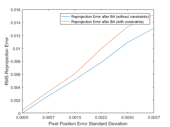
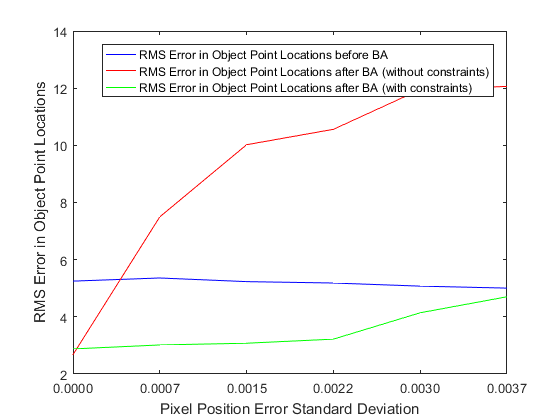
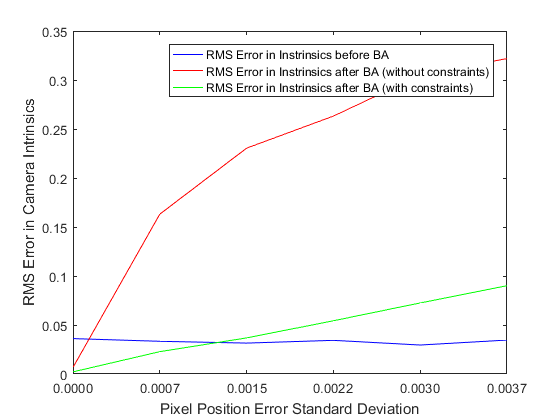

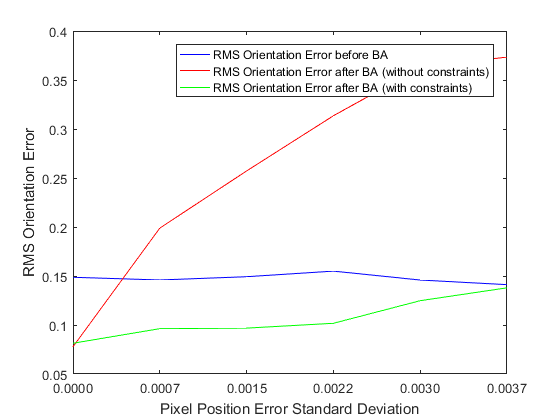
As can be seen, the constrained optimization continues to make improvements to the starting guesses for the camera parameters and object points and the amount of improvement made decreases as noise is added to the image. However, with the addition of the object point locations, the optimization is now more sensitive to image noise (particularly for the intrinsic parameters). This is expected, as the number of parameters to optimize is significantly larger.
In a practical bundle adjustment application, the number of object points and cameras would be significantly larger than that considered here, so one shouldn’t read too much into these results, however I think it is safe to conclude that:
- Adding the single camera constraint leads to significant improvement in the optimization results
- It is important to keep the image noise level low. For a 1000*1000 image, one should try to obtain features with a 1 pixel accuracy.
Exploiting the Special Structure of the Jacobian Matrix
So far, we have been solving for the parameter update by computing a direct inverse of the Hessian matrix. Doing so is both inefficient and error prone. As the size of the bundle adjustment problem gets larger, the Hessian matrix becomes more ill-conditioned. For example, the typical condition number of the Hessian matrix is ~1e -10 (calculated using rcond function in Matlab). Morever, calculating the inverse (a  operation) gets prohibitively expensive as the size of the Hessian gets larger.
Following the treatment in 1, we partition the Hessian matrix and image projection residuals as follows:
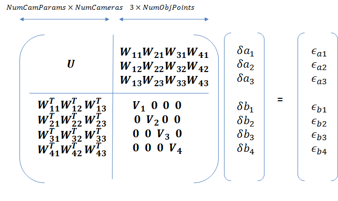
 will consist of diagonal blocks if the camera parameter blocks are independent (unconstrained optimization). When the single camera constraint is enforced, will no longer be block diagonal.
The block diagonal structure of the  arises from the fact that changing the coordinates of a 3D point only affects the image coordinates of that point and thus should always have the block diagonal structure.
Writing the equation above more compactly,

left multiplication by

yields

Since the top right block of the matrix above is 0, the dependence of the camera parameters on the structure parameters is eliminated and therefore  can be determined by solving

The matrix  is the schur compliment of and can be solved efficiently using Cholesky factorization. Once is known,
  can be obtained by solving

Solving this equation requires computing the inverse of . However due to the special structure of the bundle adjustment problem, the inverse of V is simply the concatenation of the inverses of the  block diagonal matrices:

The complexity of calculating  is thus
  where
where  is the number of object points. Since the number of object points is typically much larger than the number of cameras, this can lead to significant reduction in computation time. The condition number of the matrix is also much higher, and therefore computing the inverse of is numerically more stable than computing the inverse of the original Hessian matrix.
The Matlab code for computing the parameter updates using this method is shown below. For simplicity, we are not taking advantage of the block diagonal structure of in this code and instead computing the inverse directly.
Scaling the Image Coordinates
As noted by Haralick2, appropriately scaling the image points is critically important in obtaining a numerically stable solution for the fundamental matrix. A similar principle applies to the bundle adjustment problem. I scaled the focal length by a factor of 1000 to obtain typical image coordinates in pixel dimensions (of the order of 100s). Running the BA optimization on the scaled image coordinates produced very poor results. I then scaled the image points and the objects points as noted by Haralick such that the points are centered about the origin and the mean distance of the image points from the origin is  and that of the object points from the origin is
  . Doing so restored the numerical stability of the bundle adjustment optimization. The Matlab code for the normalization functions is shown below.
|
1 2 3 4 5 6 7 8 9 10 11 12 13 14 15 16 17 18 19 20 21 22 23 24 25 26 27 28 29 30 31 32 33 34 35 |
function [newpts, T] = normalize_3d( pts ) % Transforms 3D object points such that the points are centered about the % origin and the mean distance from the origin is sqrt(3). The function % returns the transformed points and the transformation matrix. centroid = sum(pts(:,1:3)) / size(pts,1); diff = pts(:,1:3) - repmat(centroid,size(pts,1),1); avgdist = sum(sqrt(diff(:,1).^2 + diff( :,2).^2 + diff( :,3).^2)) / size(pts,1); scale = sqrt(3) / avgdist; T = diag([scale scale scale 1]) * [eye(4,3) [-centroid 1]']; newpts = pts; newpts(:,4) = 1; newpts = newpts * T'; end function [newpts, T] = normalize_2d( pts ) % Transforms 2D image points such that the points are centered about the % origin and the mean distance from the origin is sqrt(2). The function % returns the transformed points and the transformation matrix. centroid = sum(pts(:,1:2)) / size(pts,1); diff = pts(:,1:2) - repmat(centroid,size(pts,1),1); avgdist = sum(sqrt(diff(:,1).^2 + diff( :,2).^2)) / size(pts,1); scale = sqrt(2) / avgdist; T = diag([scale scale 1]) * [eye(3,2) [-centroid 1]']; newpts = pts; newpts(:,3) = 1; newpts = newpts * T'; end |
Choosing the Right Parameterization for Rotation
In the results shown so far, we have used an axis-angle parameterization for rotation. The axis-angle representation enables a rotation to be represented by three numbers, which is the minimum required. Axis-angle representation is superior to the Euler angle representation as it doesn’t suffer from singularities. Another popular parameterization for rotation is a quaternion. A quaternion however uses 4 numbers to represent a rotation with the constraint that the norm of the quaternion is equal to 1. we implemented a version of the bundle adjustment optimization using quaternions (the major changes are that the extrinsic parameters vector is now a  vector and jacobians with respect to the quaternion elements have to be used) and found that the performance is quite poor. The reason for the poor performance is likely the extra degree of freedom introduced by using the quaternion representation. The unit norm constraint can be enforced by using lagrange parameters. Schmidt and Niemann also present a technique to enforce the unit norm constraint without using lagrange parameters3. I have not implemented this technique.
Our Bundle Adjustment vs. Matlab lsqnonlin
Matlab provides built-in implementation for many least squares optimization methods such as Levenberg-Marquardt and Trust-Region-Reflective. We compared the image reprojection errors and orientation, translation, instrinsic parameters and object point estimation errors of our BA implementation with those of Matlab. To recap, our simulation procedure is shown below.
|
1 2 3 4 5 6 7 8 9 10 11 12 13 14 15 16 17 18 19 20 21 22 23 24 25 26 27 28 29 30 31 32 33 34 35 36 37 38 39 40 41 42 43 44 45 46 47 48 49 50 51 52 53 54 55 56 57 58 59 60 61 62 63 64 65 66 67 68 69 70 71 72 73 74 |
% Simulation Procedure: % Estimated quantities are indicated by a carrot (x_c), measured quantities % by a hat (x_hat) and true values without any adornment %%%%%%%%%%%%%%%%% % Variables: %%%%%%%%%%%%%%%%% % numPoints: number of 3d object points (B). All points are visible in all % images % numCameras: number of cameras % intrinsic parameters: 3*1, focal length, image center (2*1) % extrinsic parameters: numCameras*6, 3 for rotation in axis-angle representation, 3 % for translation %%%%%%%%%%%%%%%%% % Measurements %%%%%%%%%%%%%%%%% % uv_hat = uv + randomly distributed gaussian noise with 0 mean and known % std dev. %%%%%%%%%%%%%%%%% % parameters to be estimated: %%%%%%%%%%%%%%%%% % K_c = K + estimation error in K % B_c = B + estimation error in B % For each camera % [rotation, translation]_c = [rotation, translation] + estimation error % in extrinsics % end camera % normalize all image points and object points % For increasing values of image noise std dev % do monte carlo % 1. obtain image measurements by adding normally distributed noise % with 0 mean and current std dev. % 2. obtain measurements for camera intrinsics, extrinsics and object % points by adding zero mean, constant std dev noise to the true % values. In reality, these measurements would be the output of the % previous step in 3d reconstruction pipeline % 3. Calculate estimated values of camera intrinsics, extrinsics and % object points by running the bundle adjustment optimization % 4. Calculate estimated image points by reprojecting estimated object % points using estimated camera parameters % 5. Calculate measurement residual = norm(estimated image points - % measured image points) % 6. Calculate estimation error in intrinsics, extrinsics and % object points. estimatation error = norm(estimated quantity - % true quantity) %end monte carlo % end for loop for image noise std dev |
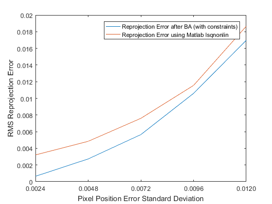
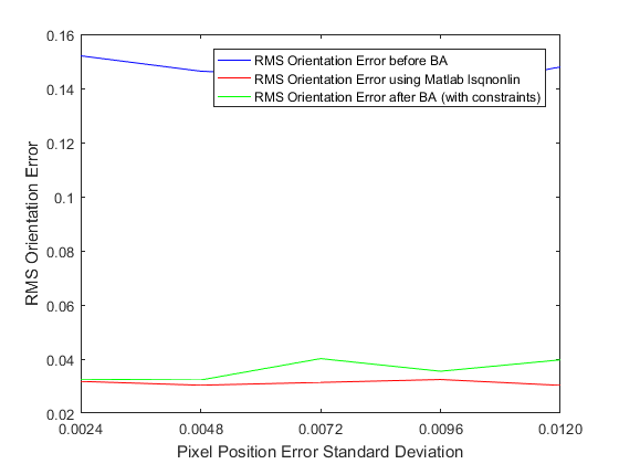
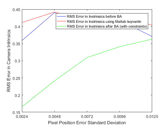
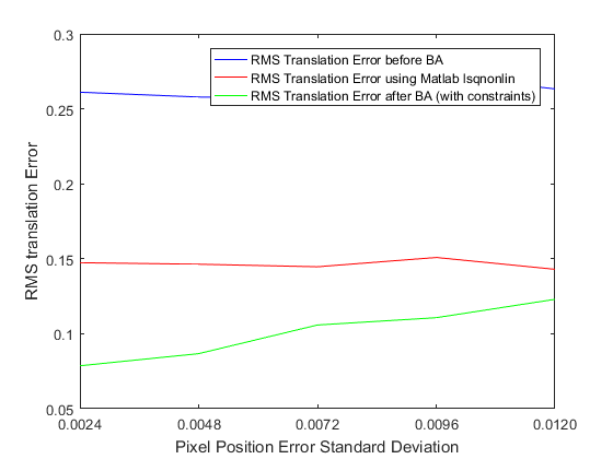
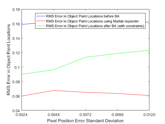
Our implementation of BA produces lower reprojection errors and performs significantly better in optimizing the camera parameters. However, Matlab’s implementation outperforms our implementation in optimizing the object point locations. One major difference between the two implementations is that Matlab’s optimization doesn’t enforce the single camera constraint. The intrinsic parameters of the optimized cameras are different from each other. Matlab’s implementation is also slower than our implementation. This could be because of the need to numerically approximate the jacobians by using numerical differentiation which leads to many more evaluations of the objective function. One shouldn’t read too much into these results however, for larger data sets, the results could be different.
Leave a Reply