
In the previous posts we considered how to calculate the Jacobians for Bundle Adjustment (BA) and their relative magnitudes and some of their properties. In this post, we’ll look at some practical implementation details of implementing BA.
Let’s quickly recap the problem we are trying to solve. Assume each camera  is parameterized by a vector
  and each 3D point
  by a vector
  . Then, Bundle Adjustment involves minimizing the following objective function:

Here,  is the predicted projection of point on the image and
  denotes the Euclidean distance between the image points represented by the vectors
  and
and  . The minimization is performed with respect to vectors and . The vector consists of the rotation and translation parameters to transform the world point in the camera coordinate system and the intrinsic parameters of the camera. The intrinsic parameters consist of the focal length (in the x and y dimensions), coordinates of the center of projection and the skew factor (if any). The vector consists of the 3D coordinates of point .
Together, these parameters are combined as follows to project a 3D world point on the image using the standard perspective projection equation.

Henceforth, we’ll assume that our camera is a rectilinear camera with square pixels. Thus,  and
and  .
.
Bundle Adjustment methods typically employ the Levenberg Marquardt (LM) algorithm to find the minimum of the optimization function. Levenberg–Marquardt algorithm solves the least squares curve fitting problem: given a set of  pairs of independent and dependent variables,
  find the parameters of the function
  so that the sum of the squares of the deviations is minimized:
![\hat{\beta} = argmin_{\beta}\sum\limits_{i=1}^m [y_i - f(x_i, \ \boldsymbol \beta) ]^2](https://telesens.co/wp-content/ql-cache/quicklatex.com-15f3818f69dd1fd71034bff1abf6cd25_l3.png "Rendered by QuickLaTeX.com")
As shown in 1, the least squares solution to this problem is obtained by solving a series of linear equations expressed in matrix form:

Here  and
and  are vectors with
  component
  and
and  respectively.
Levenberg’s contribution is to add a damping factor  to the equation above, so that we are solving:

is adjusted at each iteration. If at the end of an iteration, the objective function is lower than before, can be lowered, otherwise it is increased.
Marquardt provided the insight that we can scale each component of the gradient according to the curvature so that there is larger movement along the directions where the gradient is smaller. This avoids slow convergence in the direction of small gradient. Therefore, Marquardt replaced the identity matrix I, with a diagonal matrix consisting of the diagonal elements of  resulting in the Levenberg–Marquardt algorithm:

We’ll examine the effects of using the levenberg and Marquardt modifications when we look at our simulation results.
Let’s now examine the  matrix that arises when bundle adjustment is applied to images resulting from perspective projection. Let’s assume we have:
 3D object points
 cameras
 parameters for each camera.
To keep things simple, we’ll assume that each object point is visible in each camera (this assumption is not required and we’ll briefly consider the changes necessary to relax this assumption). The number of parameters for each camera is a combination of the camera intrinsic parameters such as camera center and focal length and extrinsic parameters such as the camera position and orientation in the world coordinate system. In our simulations, we assume that pixels are square and there is no skew. Thus the camera parameters consist of the axis-angle representation of the camera pose ( ), the camera – object translation vector (
 ) and the focal length (
 ) and camera center (
 ).
).
Let us use the following notation:
 : image coordinates of point in image (
 )
) : vector consisting of the camera parameters (
 )
) : 3D object point vector (
 )
) is the matrix consisting of the partial derivatives of the image coordinates of point in the image with the parameters of the camera
  . Thus,
  . In this post, we assume that all cameras are independent, and therefore changes in the parameters of one camera only affects the image taken by that camera, and has no effect on the other images. Therefore,
  . Each
  is a
is a  matrix laid out as follows:

The various  matrices laid out in 3D look like this:
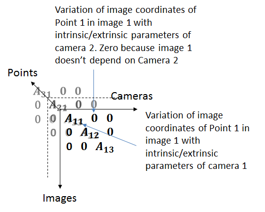
It’s easy to see that the matrix is highly sparse as changing the parameters of one camera only affects the image taken by that camera.
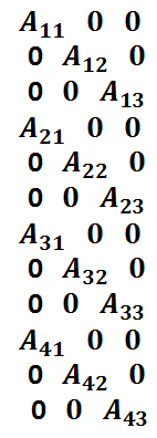
We can unroll the third dimension of the matrix and append the sub matrices corresponding to different points columnwise, so that the camera parameter part of the jacobian matrix looks like this:
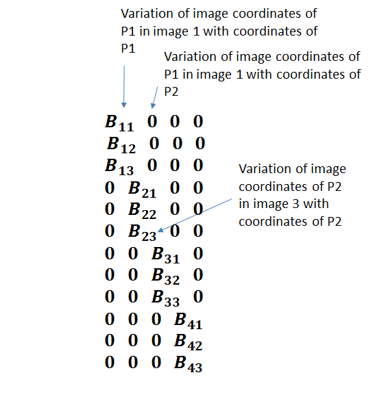
Let’s now consider the variation of image coordinates with the 3D object points.  denotes the matrix consisting of the partial derivatives of the image coordinates of point in the image with the coordinates of the object point . Thus,
  . Since change in the 3D position of one point doesn’t effect the image coordinates of another point,
  . Each
  is a
is a  matrix laid out as follows:

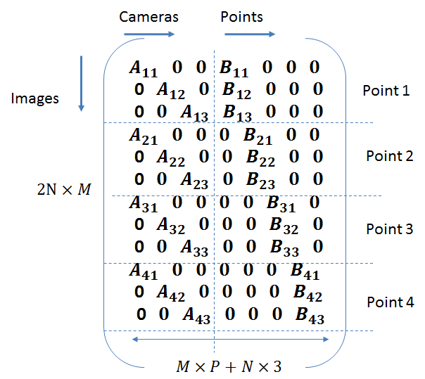
Appending the two components of the jacobian matrix, the full Jacobian matrix looks like this:
The vector  consists of the image coordinates laid out in a column vector.

Simulations
Before I describe the process and results of my simulations, let’s note one implementation detail. In my implementation, I separated the x and y components of the Jacobians so that the Jacobian matrix looks like this:
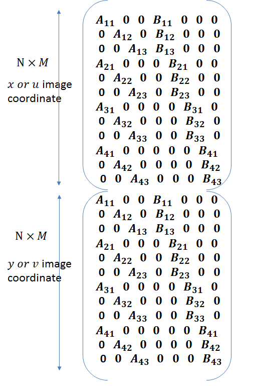 T
T
The vector also needs to be rearranged accordingly. It now looks like this:

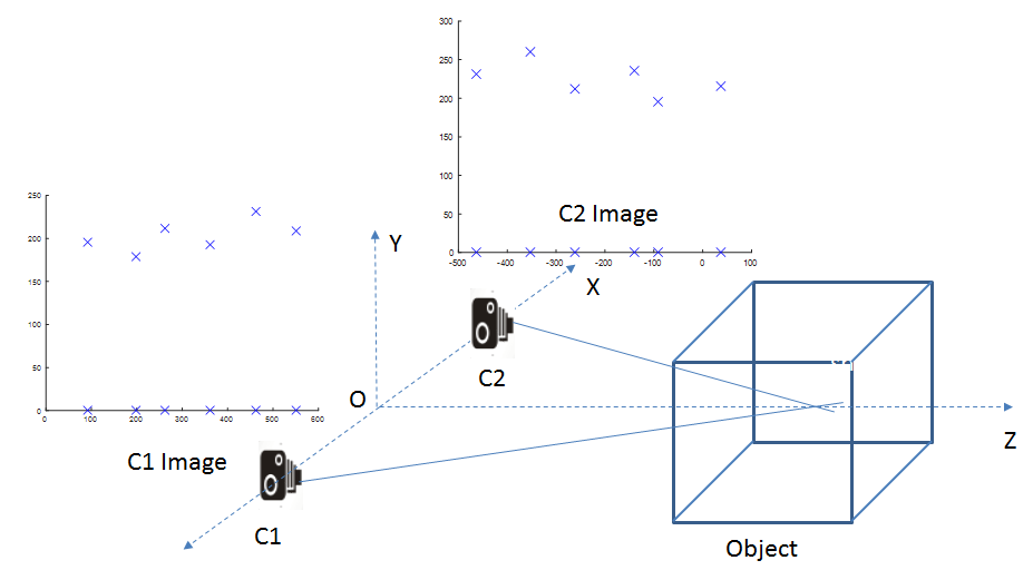
In my simulations, I considered 8 points located at the corners of a cube being viewed by multiple cameras. The set-up looks like this (only showing two cameras):
I carried out two set of simulations. In the first set, only the intrinsic and extrinsic parameters of the cameras were optimized. The position of the 3D points was not subject to the optimization. Thus, the jacobian matrix only consisted of the submatrices. In the second set, all parameters, including the position of the 3D points were part of the optimization.
Let us now look at the Matlab code for the first set.
|
1 2 3 4 5 6 7 8 9 10 11 12 13 14 15 16 17 18 19 20 21 22 23 24 25 26 27 28 29 30 31 32 33 34 35 36 37 38 39 40 41 42 43 44 45 46 47 48 49 50 51 52 53 54 55 56 57 58 59 60 61 62 63 64 65 66 67 68 69 70 71 72 73 74 75 76 77 78 79 80 81 82 83 84 85 86 87 88 89 90 91 92 93 94 95 96 97 98 99 100 101 102 103 104 105 106 107 108 109 110 111 112 113 114 115 116 117 118 119 120 121 122 123 124 125 126 127 128 129 130 131 132 133 134 135 136 137 138 139 140 141 142 143 144 145 146 147 148 149 150 151 152 153 154 155 156 157 158 159 |
function [poses, camParams] = BAImpl_NoObjPoints(objPts, poses, imgPts, f, u0, v0) % objPts is 3*numPoints numPoints = size(objPts, 2); % poses is 3*4*numCameras, each pose matrix is of the form [R T] numCameras = size(poses, 3); % wx, wy, wz, tx, ty, tz, f, u0, v0 numCamParams = 9; numJRows = 2*numPoints*numCameras; numJCols = (numCamParams*numCameras); J = zeros(numJRows, numJCols); % fill B and A B = objPts; s = 1; for i = 1:numCameras R = poses(:,1:3,i); T = poses(:, 4, i); [wx wy wz] = rotation_matrix_to_axis_angle(R); A(i,:) = [wx, wy, wz, T(1), T(2), T(3), s*f, u0, v0]; end % imgPts is a numPoints*2 vector % the "ground truth" for this optimization u_g = s*imgPts(1,:); v_g = s*imgPts(2,:); uv_g = [u_g; v_g]; uv_g = uv_g(:); err = 10000; err_prev = 10000; norm_dp = 100; numIter = 0; lambda = 0.001; % Stop the LM iteration of the norm of the change in the parameters % is less than 1.0e-6 or if numIter > 100 % just using a fixed number of iterations for now while (numIter < 80) && (norm_dp > 1e-7) && lambda < 1 numIter = numIter + 1; % Fill in the Jacobian matrix for j = 1: numCameras, wx = A(j,1); wy = A(j,2); wz = A(j,3); tx = A(j,4); ty = A(j,5); tz = A(j,6); f = A(j,7); u0 = A(j,8); v0 = A(j,9); for i = 1: numPoints, X = B(1,i); Y = B(2,i); Z = B(3,i); % x or u coordinates J((i-1)*2*numCameras+2*j-1, (j-1)*numCamParams+1: j*numCamParams) = ... [Jx_wx(X,Y,Z,f,tx,tz,u0,wx,wy,wz) Jx_wy(X,Y,Z,f,tx,tz,u0,wx,wy,wz) Jx_wz(X,Y,Z,f,tx,tz,u0,wx,wy,wz) Jx_tx(X,Y,Z,f,tz,wx,wy,wz) 0 Jx_tz(X,Y,Z,f,tx,tz,u0,wx,wy,wz) Jx_f(X,Y,Z,tx,tz,wx,wy,wz) Jx_u0 Jx_v0]; % y or v coordinates J((i-1)*2*numCameras+2*j,(j-1)*numCamParams+1:j*numCamParams) = ... [Jy_wx(X,Y,Z,f,ty,tz,v0,wx,wy,wz) Jy_wy(X,Y,Z,f,ty,tz,v0,wx,wy,wz) Jy_wz(X,Y,Z,f,ty,tz,v0,wx,wy,wz) 0 Jy_ty(X,Y,Z,f,tz,wx,wy,wz) Jy_tz(X,Y,Z,f,ty,tz,v0,wx,wy,wz) Jy_f(X,Y,Z,ty,tz,wx,wy,wz) Jy_u0 Jy_v0]; end end uv_r = computeReprojectedPts(A, B, numCameras,numPoints); d = [uv_r - uv_g]; H = J'*J; % Apply the damping factor to the Hessian matrix %H_lm=H+(lambda*eye(numJCols,numJCols)); H_lm=H+(lambda*diag(diag(H))); dp=-inv(H_lm)*(J'*d(:)); norm_dp = norm(dp); % Apply updates and compute new error. The update is contingent on % actually reducing the reprojection error A_temp = zeros(numCameras, numCamParams); for i = 1: numCameras, for j = 1: numCamParams, A_temp(i,j) = A(i,j) + dp((i-1)*numCamParams + j); end end uv_r = computeReprojectedPts(A_temp, B, numCameras,numPoints); d = [uv_r - uv_g]; err = d'*d; if (err < err_prev) lambda = lambda/2; err_prev = err; A = A_temp; else lambda = lambda*2; end end % end of Levenberg Marquardt for i = 1:numCameras R = axis_angle_to_rotation_matrix(A(i,1), A(i,2), A(i,3)); T = [A(i,4) A(i,5) A(i,6)]; poses(:, 1:3,i) = R; poses(:, 4, i) = T'; camParams(i, 1:3) = [A(i,7) A(i,8) A(i,9)]; end objPts = B; end function [u, v] = proj3dto2d(pts3d, wx, wy, wz, tx, ty, tz, f, u0, v0) % Intrinsic params matrix K = [ f 0 u0; 0 f v0; 0 0 1]; % Expression for the rotation matrix based on the Rodrigues formula R = axis_angle_to_rotation_matrix(wx, wy, wz); % Expression for the translation vector t=[tx;ty;tz]; % perspective projection of the model point (X,Y) uvs=K*[R t]*pts3d; u=uvs(1,:)./uvs(3,:); v=uvs(2,:)./uvs(3,:); end function uv_r = computeReprojectedPts(A, B, numCameras, numPoints) u_= []; v_ = []; for j = 1: numCameras, wx = A(j,1); wy = A(j,2); wz = A(j,3); tx = A(j,4); ty = A(j,5); tz = A(j,6); f = A(j,7); u0 = A(j,8); v0 = A(j,9); [u v] = proj3dto2d(B, wx, wy, wz, tx, ty, tz,f, u0, v0); u_ = [u_ u]; v_ = [v_ v]; end u_r = reshape(u_, numPoints, numCameras)'; u_r = u_r(:)'; v_r = reshape(v_, numPoints, numCameras)'; v_r = v_r(:)'; % Interleave u and vs uv_r = [u_r; v_r]; uv_r = uv_r(:); end |
Simulation Results
Let’s now look at the results of our simulations. The goal is to evaluate the relationship between image noise level and the difference between optimized camera parameters and the true camera parameters. We don’t optimize over the 3D position of the object points which are assumed to be known with high accuracy. This scenario models the optimization carried out during camera calibration, where the position of the object points (corners of the calibration pattern) is known through direct measurements. One difference between the camera calibration scenario and this simulation is that it is customary to use a planar calibration pattern during camera calibration, and thus the image coordinates on different images of the pattern are related to each other by a homography. In our simulation, the object points are non-coplanar and their image coordinates follow the epipolar constraint and are not related by a homography.
We expect that as noise is added to the image, the distance between the optimized camera parameters and the true parameters would increase. This is indeed borne out by our simulation, as shown in the plots below.
The pseudo-code for the simulation is shown below.
|
1 2 3 4 5 6 7 8 9 10 11 12 13 14 15 16 17 18 19 20 21 22 23 24 25 26 27 28 29 30 31 32 33 34 35 36 37 38 39 40 41 42 43 44 45 46 47 |
maxDim = max(imgWidth, imgHeight) % One can typically obtain the position of image features to sub-pixel accuracy. % For a 1024 by 1024 image, a dislocation by 1 pixel amounts to roughly adding % noise of std-dev of 0.001. This is the basis of choosing the std deviation % numbers shown below image_noise_std_dev = [0 0.001*maxDim 0.002*maxDim 0.003*maxDim 0.004*maxDim ... 0.005*maxDim]; % We use a standard deviation of 5 degrees for error in the orientation, % 5 units for error in the translation (amounting to roughly a 10% error in the translation) % and 3% error in the camera intrinsic parameters. Samples will be drawn from a Gaussian distribution % centered around the true value of the parameters with these standard deviations. These samples will % serve as the starting point for the bundle adjustment optimization. camera_params_noise_std_dev = [5*DEGTORAD, 5*DEGTORAD, 5*DEGTORAD, 5, 5, 5, maxDim*0.03, maxDim*0.03, maxDim*0.03]; % No noise is added to the object points, which are assumed to be known with high % accuracy for img_std_dev in image_noise_std_dev -run montecarlo analysis (50 samples) - add randomly distributed noise according to img_std_dev to image coordinates - add randomly distributed noise to orientation, translation and intrinsic camera parameters - calculate RMS error between noisy and un-corrupted orientation/translation/intrinsics. - This is the error in orientation/translation/intrinsics before optimization - Run unconstrained bundle adjustment with the noisy orientation/translatoin/intrinsics - as starting point and with the noisy image coordinates. - Calculate RMS error between original and optimized parameters. Also calculate - Reprojection error using the optimized parameters. - Repeat for constrained bundle adjustment -end monte carlo -end image_noise_std_dev loop Plot reprojection error, RMS errors in orientation/translation/intrinsics |
In our simulations, we use points located on the corners of 3 planes displaced from each other by a fixed distance, leading to 12 points in total. These points are viewed by 4 cameras. The view from one of the cameras is shown below.
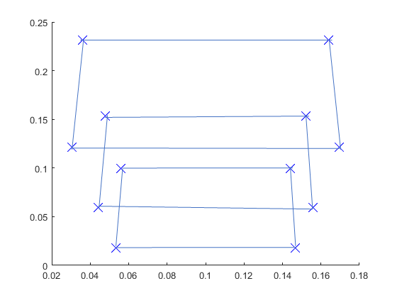
No image space scaling or clipping is applied and all points are assumed to be visible from all 4 poses. Since no image space scaling is applied, the image coordinates are numerically much smaller than they normally are (of the order of 0.1 instead of 100’s).
The number of independent equations are 2*12*4 = 96, while the number of parameters are 4*9 = 36 (6 extrinsic and 3 intrinsic parameters for each camera).
Calculating the RMS Errors
Denoting the optimized value of parameter P by  and original value by
  , the RMS error is given by:

For orientation, the rotation error matrix is first calculated ( ) and the error matrix is converted into the axis-angle representation. The axis-angle vector is then used as a regular vector in the expression for RMS error above.
Simulation Results
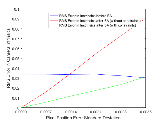
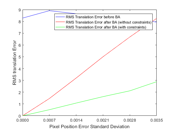
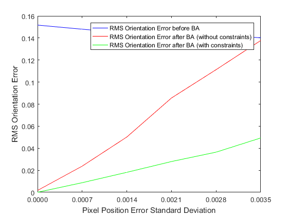
As we can see, the error in the estimated intrinsic and extrinsic parameters increases with the standard deviation of the image noise. However even in the presence of significant noise, bundle adjustment makes improvements to the original estimate of the extrinsic and intrinsic parameters.
Constrained Optimization
In our formulation of Bundle Adjustment, we treat each camera as independent and hence the optimization converges to different values of the extrinsic and intrinsic parameters for each camera. However, in the vast majority of use cases, a single camera is used to capture multiple images from different poses. The extrinsic parameters for these poses are different, but the intrinsic parameters are the same. Thus, it would make sense to modify the Jacobian matrix to add this additional constraint. The constraint is enforced by recognizing that the image coordinates in all images vary with the a change in the intrinsic parameters, not just the coordinates in a particular image.
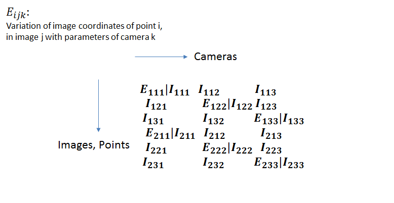
In the figure above, we have broken an individual jacobian entry into its extrinsic and intrinsic component, and also shown the point, image and camera indicies separately. The variation of the image coordinates with the object points () don’t change.
Adding this constraint leads to significant improvements in the minimum achieved by the optimization, as shown in the plots above. The improvement is particularly significant for the camera intrinsic parameters. The unconstrained optimization ceases to make improvements to the initial guess for the intrinsic parameters, even in the presence of a small amount of noise, whereas the constrained optimization continues to make improvements.
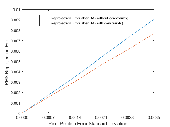
Reprojection Error
As shown in the graph above, the constrained optimization performs better than the unconstrained optimization in minimizing the reprojection error. Indeed, the reprojection error achieved by the constrained optimization is often lower than the “best case” reprojection error, which is calculated by using the image coordinates obtained by projecting the object points using the correct pose and the noisy image points. It is possible for the overall reprojection error to be lower for poses different from the “correct” poses depending on the geometry at hand.
Relative Values of the Orientation/Translation/Intrinsics Jacobians
In this section, I’ll attempt to provide some insights on the relative values of the jacobians of the orientation, translation and intrinsic parameters. Consider a point  with coordinates
  in the local object coordinate system. For simplicity, we’ll assume that the object coordinate system is aligned with the camera coordinate system and there is a translation of
  between the two coordinate systems. Let’s also assume that the camera under consideration is a normalized camera with focal length and image center =
  . The image coordinates of are given by:


From the figure below,


For simplicity, let’s represent the rotation of the object coordinate system by Euler angles, with  denoting the angle of rotation about the
  axes. Let’s consider the first row of Jacobian matrix of the camera parameters.

Considering only the rotation about the y axis (the analysis of rotation about other axes is similar),

= 
Now let’s consider the first row of the Jacobian of the Object points. Denoting the coordinates of in the camera coordinate system by  ,
,

From these numbers, we can make the following observations:
- The sensitivity of the image coordinates to the intrinsic parameters is much higher than to the rotation and translation parameters. Among the intrinsic parameters, the image center is the most important.
- The sensitivity of the image coordinates to the rotation parameters depends upon the angle of rotation. The sensitivity to rotation is lowest for glancing angles (when
 ).
). - The sensitivity of the image coordinates to the object coordinates is of the same order as that to the camera-object translation.
These observations are verified by the actual Jacobian values in our simulations.
Levenberg-Marquardt Optimization
Lastly, we’ll consider the effect of the Levenberg and Marquardt modifications used in the Levenberg Marquardt optimization. Recall that Levenberg contribution was to introduce a damping factor that is increased or decreased after every iteration depending upon whether the objective function is higher or lower than in the previous iteration. Marquardt added a term to scale each component of the gradient so that there is larger movement along the direction where the gradient is smaller. The number of iterations the optimization takes to converge with these improvements is shown in the table below:
| Optimization | Number of Iterations |
| No optimization | 1200 |
| Levenberg Improvement | 20 |
| Marquardt Improvement | 9 |
From this table it is clear that the Levenberg-Marquardt improvements have a significant impact on the speed of convergence. The Marquardt improvement also helps the optimizations avoid local minimums that result from the interplay between focal length and the z component of the translation vector. For some orientations, similar amounts of reduction in the objection function can be achieved by either decreasing/increasing the z component of the translation vector or decreasing/increasing the focal length. The Marquardt optimization discourages the optimization from favoring changes in focal length over changes in the translation.
In the next post, we’ll consider the second second of simulations, where we also optimize over the positions of the 3D object points.
Leave a Reply