Bundle Adjustment – Part 2: Jacobians

In the previous post, we considered the basics of bundle adjustment (BA) and discussed how to obtain the expressions for the jacobian matrices for the case of perspective projection. Let’s now look at these expressions in more detail.

Dependencies

The table below lists the parameters each element of the jacobian matrix depends on. Jx_wx denotes the partial derivative of the x image coordinate wrt to wx.

Jx_wx	Jx_wx(X,Y,Z,f,tx,tz,u0,wx,wy,wz)
Jx_wy	Jx_wx(X,Y,Z,f,tx,tz,u0,wx,wy,wz)
Jx_wz	Jx_wx(X,Y,Z,f,tx,tz,u0,wx,wy,wz)
Jx_tx	Jx_tx(X,Y,Z,f,tz,wx,wy,wz)
Jx_ty	0
Jx_tz	Jx_tz(X,Y,Z,f,tx,tz,u0,wx,wy,wz)
Jx_f	Jy_f(X,Y,Z,ty,tz,wx,wy,wz)
Jx_u0	1
Jx_v0	1
Jx_X	Jx_X(X,Y,Z,f,tx,tz,u0,wx,wy,wz)
Jx_Y	Jx_Y(X,Y,Z,f,tx,tz,u0,wx,wy,wz)
Jx_Z	Jx_Z(X,Y,Z,f,tx,tz,u0,wx,wy,wz)

From this table, we can make the following observations.

Because we assumed zero skew, the variables along the x and y axis do not have any cross-depenencies.
The jacobian of the focal length doesn’t depend on the value of the focal length
The jacobians of the image center are constants

These results agree with expressions for the jacobians we obtained in the previous post where we considered the object point in the camera coordinate system and thus avoided the complexity introduced by the object-camera coordinate system transformation.

The table above shows the variation of the x component of the Jacobian. The y component follows the same pattern with x, y and u, v interchanged.

Verifying the Jacobians are Correct

If you look at the Matlab files containing the implementation of the different elements of the Jacobian matrix (generated by the “matlabFunction” function) you’ll notice that the expressions are very complex. So how to do we know that these expressions are actually correct?

I verified the accuracy of the jacobians by comparing the output of the jacobian function with that calculated manually by numerical differentiation. The code for the variation of Jx_wx is shown below:

for wx_val = wx - 5:dwx:wx + 5,
    [u v] = proj3dto2d(pts3d, wx_val, wy, wz, tx, ty, tz, f, u0, v0);
    % compute the value of the derivative manually
    du_dwx = (u - u_prev)/dwx;
    u_prev = u;
    % compute the value from the jacobian
    Jx_wx_arr(end+1) = Jx_wx(X, Y, Z, f, tx, tz, u0, wx_val, wy, wz);
    du_dwx_arr(end+1) = du_dwx;
    R = axis_angle_to_rotation_matrix(wx_val, wy, wz);
    u_arr(end+1) = u;
end

for wx_val = wx - 5:dwx:wx + 5,

[u v] = proj3dto2d(pts3d, wx_val, wy, wz, tx, ty, tz, f, u0, v0);

% compute the value of the derivative manually

du_dwx = (u - u_prev)/dwx;

u_prev = u;

% compute the value from the jacobian

Jx_wx_arr(end+1) = Jx_wx(X, Y, Z, f, tx, tz, u0, wx_val, wy, wz);

du_dwx_arr(end+1) = du_dwx;

R = axis_angle_to_rotation_matrix(wx_val, wy, wz);

u_arr(end+1) = u;

end

The plot below shows the derivative from numerical computation and the derivative from the jacobian plotted against the independent variable (wx). The other variables that the Jacobian depends upon (X,Y,X, f etc) were kept constant.

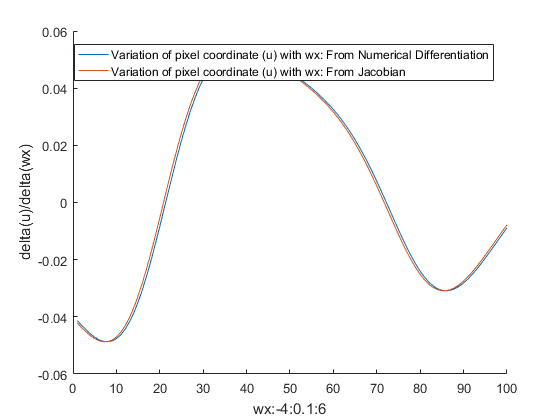
One can see that the derivative from numerical computation is in close agreement with that computed from the jacobian.

Relationship between axis-angle representation and Rotation Matrix representation

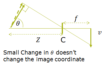
As noted in the previous post, we use the axis-angle representation to represent rotations because it is a compact representation and captures the angle and axis of rotation by 3 numbers denoted by $w = (w_x, w_y, w_z)$ . In the axis-angle representation, the angle of rotation is represented by $\|w\|$ while $\frac{w}{\|w\|}$ represents the unit vector corresponding to the axis of rotation. The axis-angle rotation is superior to the more commonly used euler angle representation as it doesn’t suffer from gimbal lock. The relationship between the two representations is quite non-linear. The graphs below show the variation of yaw, pitch and roll when $w_x$ is varied from -4 to 6.

We can see that linearly varying one coordinate of the axis-angle representation changes all three euler angles in a highly non-linear way.

Lastly, let’s look at some plots of the variation of some of these Jacobians.

Variation of $J_xt_z$ and $J_xt_x$

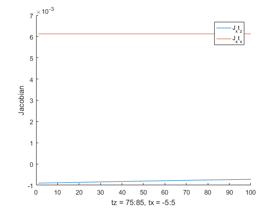
This plot was obtained by varying tx and tz around the mid point values of 0 and 80. The numbers on the x-axis are just array indicies, not parameter values since the x-axis for the two plots represent two different variables – tx and ty. The 3D coordinates of the point under consideration is X, Y, Z = 10, 10, 10. The plot verifies the observations made in the previous post:

$J_xt_x$ doesn’t vary with tx
$J_xt_x$ is roughly 7 times the value of $J_xt_z$ , which is approximately equal to the ratio of Z and X of the 3D point in the camera coordinate system
$J_xt_z$ varies inversely with $t_z$ (the variation is inverse square, but that is hard to see in the plot as the values of $J_xt_z$ ) are quite small. This agrees with our intuitive understanding that depth perception becomes harder as the object moves farther from the camera.

Variation of $J_xf$

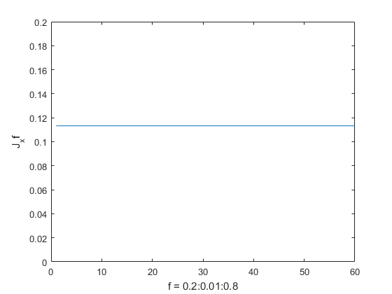
The plot below shows the variation of $J_xf$ with the focal length. All other variables are kept constant ( $X=Y=Z=10, t_x, t_y = 0, t_z=80$ ). As expected, $J_xf$ does not change with $f$ and the value of the jacobian is approximately $\frac{X}{f} \approx 20$ times that of $J_xt_x$ .

Variation of $J_xw_x, J_xw_y, J_xw_z$

The plot below shows the rotation elements of the Jacobian. It’s important to note that the Jacobians vary a lot, and for certain rotations, some of the Jacobians become zero. I suspect this occurs when the angle of rotation is such that the line of sight from the camera is a tangent to the direction of rotation.

Telesens

Bundle Adjustment – Part 2: Jacobians

Be the first to comment

Leave a Reply Cancel reply